# TensorFlow Examples

# Linear Regression

# Example 01

Importing labraries:

import numpy as np
import matplotlib.pyplot as plt
import tensorflow as tf

1
2
3

Data generation

To generate the data necessary we create random numbers between -10 and 10 for xs and zs as well as our noise, between -1 and 1. In a total of 1000 observations each.

Then we create a generated_inputs by stacking xs and zs in a np.column_stack.

The generated_targets will be the function we want to achieve.

Finally, we save then into a tensor friendly np.savez file.

TIP

Running this code will generate the .npz file in the projects folder.

observations = 1000

xs = np.random.uniform(low=-10, high=10, size=(observations, 1))
zs = np.random.uniform(-10, 10, (observations, 1))

generated_inputs = np.column_stack((xs, zs))

noise = np.random.uniform(-1, 1, (observations, 1))

generated_targets = 2*xs - 3*zs + 5 + noise

np.savez(inputs=generated_inputs, targets=generated_targets)

1
2
3
4
5
6
7
8
9
10
11
12
13

Solving with TensorFlow

First we load the .npz file, the we create a input_size variable equal to 2 (xs and zs) and an output_size variable = 1 (y).

Our algorithm has a simple structure, it takes inputs applies a single linear transformation and provides outputs. For this we are going to use the Dense from tf.keras.

TIP

Basically it takes the inputs provided to the model and calculates the dot product of the inputs and the weights and adds the bias.

Dense implements the operation: output = activation(dot(input, kernel) + bias) where activation is the element-wise activation function passed as the activation argument, kernel is a weights matrix created by the layer, and bias is a bias vector created by the layer (only applicable if use_bias is True).

model = tf.keras.Sequential([tf.keras.layers.Dense(output_size)])

Compile the Sequential model created with the unique layer

sgd = stochastic gradient descent tf.keras.optimizers

L2-norm loss = Least sum of squares (least sum of squared error). Scaling by #observations = average(mean), so we can use mean_squared_error(...) (tf.keras.losses.MSE)

model.compile(optimizer='sgd', loss='mean_squared_error')

The last step is to indicated to the model which data to fit.

model.fit(training_data['inputs'], training_data['targets'], epochs=100, verbose=0)

When we run we can see the epochs:

Epoch 1/100
 1/32 [..............................] - ETA: 0s - loss: 177.1277
32/32 [==============================] - 0s 1ms/step - loss: 21.6579
Epoch 2/100
32/32 [==============================] - 0s 468us/step - loss: 4.3905
Epoch 3/100
32/32 [==============================] - 0s 469us/step - loss: 1.4498
Epoch 4/100
32/32 [==============================] - 0s 469us/step - loss: 0.6680
Epoch 5/100
32/32 [==============================] - 0s 531us/step - loss: 0.4313
0s 407us/step - loss: 0.3444
.
.
.
Epoch 95/100
32/32 [==============================] - 0s 375us/step - loss: 0.3451
Epoch 96/100
32/32 [==============================] - 0s 437us/step - loss: 0.3430
Epoch 97/100
32/32 [==============================] - 0s 406us/step - loss: 0.3427
Epoch 98/100
32/32 [==============================] - 0s 406us/step - loss: 0.3447
Epoch 99/100
32/32 [==============================] - 0s 437us/step - loss: 0.3413
Epoch 100/100
32/32 [==============================] - 0s 438us/step - loss: 0.3414

1
2
3
4
5
6
7
8
9
10
11
12
13
14
15
16
17
18
19
20
21
22
23
24
25
26
27

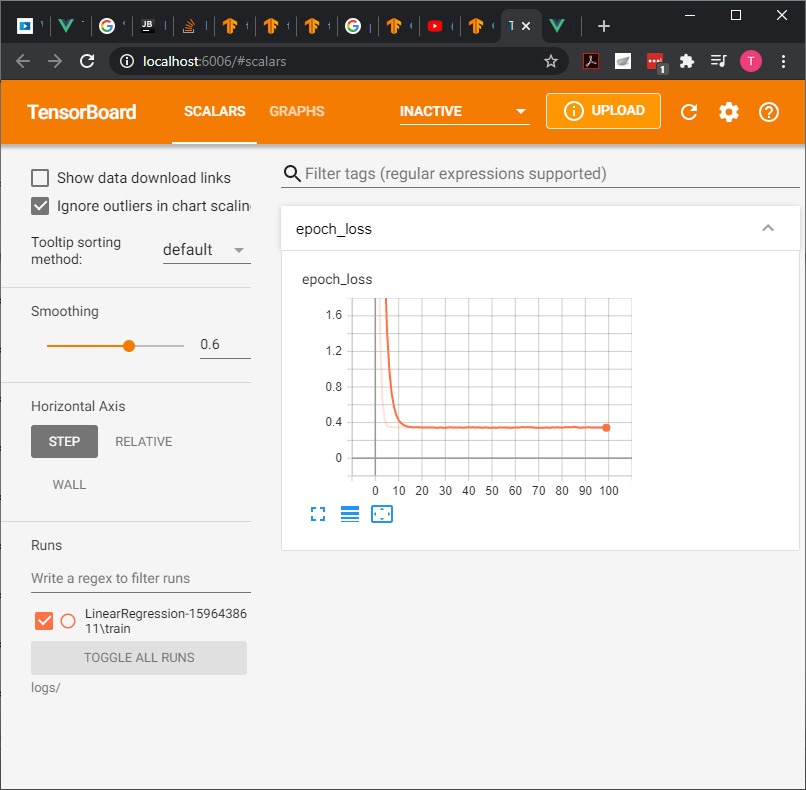
Using TensorBoard

To use TensorBoard we have to include:

import time
from tensorflow.keras.callbacks import TensorBoard

NAME = "LinearRegression-{}".format(int(time.time()))
tensorboard = TensorBoard(log_dir='logs/{}'.format(NAME))

1
2
3
4
5

Then, on the model.fit, we include the callback

model.fit(training_data['inputs'], training_data['targets'],
 epochs=100, verbose=1, callbacks=[tensorboard])

1
2

In the terminal call tensorboard

tensorboard --logdir logs/

Extract the weights and bias

Weights:

weights = model.layers[0].get_weights()[0]
print("weights = ", weights)

1
2

weights =  [[ 1.9636236]
 [-3.0029242]]

1
2

bias = model.layers[0].get_weights()[1]
print("bias = ", bias)

1
2

bias =  [5.013836]

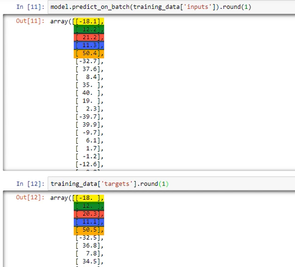
Extract the outputs (make predictions)

The result is an array with the corresponding outputs for each of the inputs.

model.predict_on_batch(training_data['inputs'])

array([[ 2.20054913e+00],
       [ 3.50056305e+01],
       [-7.09030628e+00],
       [ 1.26977491e+01],
       [ 1.12016077e+01],
       [-2.65325775e+01],
       [ 2.31708298e+01],
       [ 1.28329201e+01],
       [ 5.50317049e+00],
       [ 3.25315819e+01],
       [-1.00832729e+01],
       [-1.62092972e+00],
.
.
.
       [-9.93519592e+00],
       [ 1.90676994e+01],
       [ 1.92885208e+01],
       [-4.08601856e+00],
       [-4.01976051e+01],
       [-1.64834194e+01],
       [-9.02546692e+00],
       [-1.77080956e+01]], dtype=float32)

1
2
3
4
5
6
7
8
9
10
11
12
13
14
15
16
17
18
19
20
21
22
23

We can round the results for better visualization:

model.predict_on_batch(training_data['inputs'])
model.predict_on_batch(training_data['inputs']).round(1)

1
2

If we compare the prediction of the inputs with the targets they will look very close:

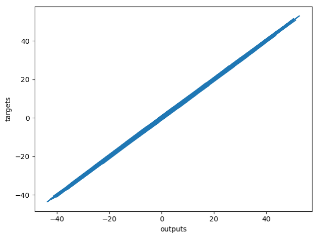
Plot

plt.plot(np.squeeze(model.predict_on_batch(training_data['inputs'])), np.squeeze(training_data['targets']))
plt.xlabel('outputs')
plt.ylabel('targets')
plt.show()

1
2
3
4