# R

# Resources

# Introduction

R uses functions to perform operations. To run a function called funcname, we type funcname(input1, input2), where the inputs (or arguments) input1 argument and input2 tell R how to run the function.

A function can have any number of inputs. For example, to create a vector of numbers, we use the function c() (for concatenate). Any numbers inside the parentheses are joined together. The following command instructs R to join together the numbers 1, 3, 2, and 5, and to save them as a vector named x. When we type x, it vector gives us back the vector.

> x <- c(1,3,2,5)
> x
[1] 1 3 2 5

1
2
3

or we can use "="

> x = c(1,3,2,6)
> x
[1] 1 3 2 6

1
2
3

In addition, typing ?funcname will always cause R to open a new help file window with additional information about the function funcname.

We can tell R to add two sets of numbers together. It will then add the first number from x to the first number from y, and so on. However, x and y should be the same length. We can check their length using the length() function.

> length(x)
[1] 4
> y = c(1,4,3)
> length(y)
[1] 3
> x + y
[1] 2 7 5 7
Warning message:
In x + y : longer object length is not a multiple of shorter object length
> x = c(1,6,2)
> x + y
[1]  2 10  5

1
2
3
4
5
6
7
8
9
10
11
12

The ls() function allows us to look at a list of all of the objects, such as data and functions, that we have saved so far. The rm() function can be used to delete any that we don’t want.

> ls()
[1] "x" "y"
> rm(x,y)
> ls()
character(0)

1
2
3
4
5

It’s also possible to remove all objects at once:

> x = c(1,6,2)
> y = c(1,4,3)
> ls()
[1] "x" "y"
> rm(list=ls())
> ls()
character(0)

1
2
3
4
5
6
7

The matrix() function can be used to create a matrix of numbers. Before we use the matrix() function, we can learn more about it:

> ?matrix

The help file reveals that the matrix() function takes a number of inputs, but for now we focus on the first three: the data (the entries in the matrix), the number of rows, and the number of columns.

First, we create a simple matrix.

> x=matrix(data=c(1,2,3,4), nrow =2, ncol=2)
> x
     [,1] [,2]
[1,]    1    3
[2,]    2    4

1
2
3
4
5

Note that we could just as well omit typing data=, nrow=, and ncol= in the matrix() command above: that is, we could just type:

> x=matrix (c(1,2,5,8) ,2,2)
> x
     [,1] [,2]
[1,]    1    5
[2,]    2    8

1
2
3
4
5

and this would have the same effect. However, it can sometimes be useful to specify the names of the arguments passed in, since otherwise R will assume that the function arguments are passed into the function in the same order that is given in the function’s help file.

As this example illustrates, by default R creates matrices by successively filling in columns. Alternatively, the byrow=TRUE option can be used to populate the matrix in order of the rows.

> matrix (c(1,2,3,4) ,2,2,byrow =TRUE)
     [,1] [,2]
[1,]    1    2
[2,]    3    4

1
2
3
4

Notice that in the above command we did not assign the matrix to a value such as x. In this case the matrix is printed to the screen but is not saved for future calculations. The sqrt() function returns the square root of each element of a vector or matrix. The command x^2 raises each element of x to the power 2; any powers are possible, including fractional or negative powers.

> x
     [,1] [,2]
[1,]    1    5
[2,]    2    8

1
2
3
4

> sqrt(x)
         [,1]     [,2]
[1,] 1.000000 2.236068
[2,] 1.414214 2.828427

1
2
3
4

> x^2
     [,1] [,2]
[1,]    1   25
[2,]    4   64

1
2
3
4

The rnorm() function generates a vector of random normal variables, with first argument n the sample size. Each time we call this function, we will get a different answer.

Here we create two correlated sets of numbers, x and y, and use the cor() function to compute the correlation between them.

> x=rnorm (50)
> x
 [1]  0.60366801  0.25451607 -0.88203475  1.50833657 -0.86380284  0.40682715 -0.90281982
 [8]  0.28111844 -0.02906223  0.44137641  1.28192379  0.25212626 -0.90114271  0.07013796
[15] -0.01819873  0.02925782 -0.66536433  1.03774640 -0.16331192  0.73054311 -0.33181742
[22] -0.53952808 -0.77753887  0.09671780 -1.69165908  2.18654439 -0.76772002  1.41926783
[29]  0.69901969 -0.73841653 -0.33519705  0.89284669  0.46658627 -0.80923650  0.44937484
[36] -0.98993311  0.72273524  0.81736489  0.20818078  1.06483904  0.78438860  0.79083635
[43]  0.56856373  1.03840099 -1.10476512 -0.24643069 -1.83372730  0.42040382 -1.24376742
[50] -0.25049661
> y=x+rnorm (50, mean=50, sd=.1)
> y
 [1] 50.52346 50.23295 48.96515 51.43617 49.08099 50.42082 49.01942 50.38520 50.09021
[10] 50.40177 51.36268 50.18730 48.99076 49.91912 50.07773 50.00302 49.27951 50.81956
[19] 49.81580 50.88197 49.64394 49.19755 49.05280 50.05001 48.21460 52.34628 49.30141
[28] 51.42377 50.80615 49.15450 49.63649 50.90449 50.44182 49.35922 50.40463 48.94124
[37] 50.77157 50.76696 50.18971 51.07317 50.82507 50.87767 50.46613 51.09629 49.05959
[46] 49.54172 48.24741 50.23709 48.74109 49.69187
> cor(x,y)
[1] 0.9935359

1
2
3
4
5
6
7
8
9
10
11
12
13
14
15
16
17
18
19
20

By default, rnorm() creates standard normal random variables with a mean of 0 and a standard deviation of 1. However, the mean and standard deviation can be altered using the mean and sd arguments, as illustrated above.

Sometimes we want our code to reproduce the exact same set of random numbers; we can use the set.seed() function to do this. The set.seed() function takes an (arbitrary) integer argument.

> set.seed (1303)
> rnorm(50)
 [1] -1.1439763145  1.3421293656  2.1853904757  0.5363925179  0.0631929665  0.5022344825
 [7] -0.0004167247  0.5658198405 -0.5725226890 -1.1102250073 -0.0486871234 -0.6956562176
[13]  0.8289174803  0.2066528551 -0.2356745091 -0.5563104914 -0.3647543571  0.8623550343
[19] -0.6307715354  0.3136021252 -0.9314953177  0.8238676185  0.5233707021  0.7069214120
[25]  0.4202043256 -0.2690521547 -1.5103172999 -0.6902124766 -0.1434719524 -1.0135274099
[31]  1.5732737361  0.0127465055  0.8726470499  0.4220661905 -0.0188157917  2.6157489689
[37] -0.6931401748 -0.2663217810 -0.7206364412  1.3677342065  0.2640073322  0.6321868074
[43] -1.3306509858  0.0268888182  1.0406363208  1.3120237985 -0.0300020767 -0.2500257125
[49]  0.0234144857  1.6598706557

1
2
3
4
5
6
7
8
9
10
11

We use set.seed() throughout the labs whenever we perform calculations involving random quantities. In general this should allow the user to reproduce our results. However, it should be noted that as new versions of R become available it is possible that some small discrepancies may form between the book and the output from R.

The mean() and var() functions can be used to compute the mean and variance of a vector of numbers. Applying sqrt() to the output of var() will give the standard deviation. Or we can simply use the sd() function.

> set.seed (3)
> y-rnorm(100)
  [1] 51.48540 50.52547 48.70636 52.58830 48.88521 50.39069 48.93400 49.26859 51.30907
 [10] 49.13440 52.10746 51.31851 49.70712 49.66647 49.92568 50.31067 50.23253 51.46781
 [19] 48.59148 50.68216 50.22243 50.13985 49.25653 51.71649 48.69905 53.08735 48.14079
 [28] 50.41171 50.87823 50.29128 48.73587 50.05272 49.71410 48.62272 50.75676 48.23572
 [37] 49.47121 50.72871 51.16900 50.27941 50.03857 51.18813 48.76725 51.89088 48.71115
 [46] 51.80712 48.40961 49.10622 49.19664 50.59104 49.79662 51.04239 48.69806 53.17343
 [55] 50.49241 50.87437 50.05491 49.02306 49.17275 51.18691 50.78916 49.26910 48.73447
 [64] 49.56715 48.90339 50.48386 49.69834 49.86445 51.10480 50.69577 49.67527 48.73045
 [73] 48.02860 49.78266 47.98277 51.59869 48.08434 51.04041 51.79420 49.31135 47.90096
 [82] 51.25678 49.75318 48.13481 49.61033 48.94764 50.55242 51.65343 49.74995 51.95956
 [91] 51.67889 51.86766 51.11701 50.04234 49.45047 49.61231 48.70946 49.69618 47.80946
[100] 49.90115
> mean(y)
[1] 50.04716
> var(y)
[1] 0.7919301
> sqrt(var(y))
[1] 0.8899045
> sd(y)
[1] 0.8899045

1
2
3
4
5
6
7
8
9
10
11
12
13
14
15
16
17
18
19
20
21
22

# Graphics

The plot() function is the primary way to plot data in R. For instance, plot(x,y) produces a scatterplot of the numbers in x versus the numbers in y. There are many additional options that can be passed in to the plot() function. For example, passing in the argument xlab will result in a label on the x-axis. To find out more information about the plot() function, type ?plot.

> x=rnorm (100)
> y=rnorm (100)
> plot(x,y)

1
2
3

> plot(x,y, xlab="this is the x-axis",ylab="this is the yaxis", main="Plot of X vs Y")

We will often want to save the output of an R plot. The command that we use to do this will depend on the file type that we would like to create. For instance, to create a pdf, we use the pdf() function, and to create a jpeg, we use the jpeg() function.

> pdf (" Figure.pdf ")
> plot(x,y,col =" green ")
> dev.off()
RStudioGD 
        2

1
2
3
4
5

The function dev.off() indicates to R that we are done creating the plot. Alternatively, we can simply copy the plot window and paste it into an appropriate file type, such as a Word document.

The function seq() can be used to create a sequence of numbers. For instance, seq(a,b) makes a vector of integers between a and b. There are many other options: for instance, seq(0,1,length=10) makes a sequence of 10 numbers that are equally spaced between 0 and 1. Typing 3:11 is a shorthand for seq(3,11) for integer arguments.

> x=seq(1,10)
> x
 [1]  1  2  3  4  5  6  7  8  9 10
> x=1:10
> x
 [1]  1  2  3  4  5  6  7  8  9 10
> x=seq(-pi,pi,length=50)
> x
 [1] -3.14159265 -3.01336438 -2.88513611 -2.75690784 -2.62867957 -2.50045130 -2.37222302
 [8] -2.24399475 -2.11576648 -1.98753821 -1.85930994 -1.73108167 -1.60285339 -1.47462512
[15] -1.34639685 -1.21816858 -1.08994031 -0.96171204 -0.83348377 -0.70525549 -0.57702722
[22] -0.44879895 -0.32057068 -0.19234241 -0.06411414  0.06411414  0.19234241  0.32057068
[29]  0.44879895  0.57702722  0.70525549  0.83348377  0.96171204  1.08994031  1.21816858
[36]  1.34639685  1.47462512  1.60285339  1.73108167  1.85930994  1.98753821  2.11576648
[43]  2.24399475  2.37222302  2.50045130  2.62867957  2.75690784  2.88513611  3.01336438
[50]  3.14159265

1
2
3
4
5
6
7
8
9
10
11
12
13
14
15
16

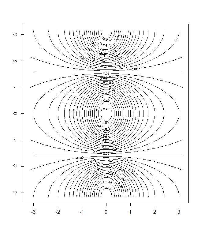
We will now create some more sophisticated plots. The contour() function produces a contour plot in order to represent three-dimensional data; it is like a topographical map. It takes three arguments:

A vector of the x values (the first dimension),
A vector of the y values (the second dimension), and
A matrix whose elements correspond to the z value (the third dimension) for each pair (x,y) coordinates.

As with the plot() function, there are many other inputs that can be used to fine-tune the output of the contour() function. To learn more about these, take a look at the help file by typing ?contour.

> y=x
> f=outer(x,y,function (x,y)cos(y)/(1+x^2))
> f=outer(x,y,function (x,y)cos(y)/(1+x^2))
> contour(x,y,f)

1
2
3
4

> contour (x,y,f,nlevels =45, add=T)

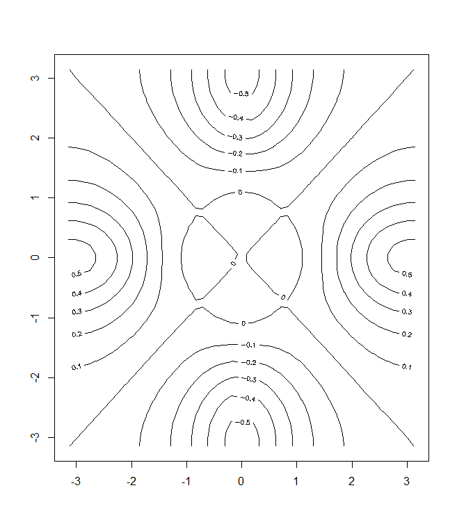
> fa=(f-t(f))/2
> contour (x,y,fa,nlevels =15)

1
2

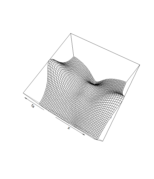
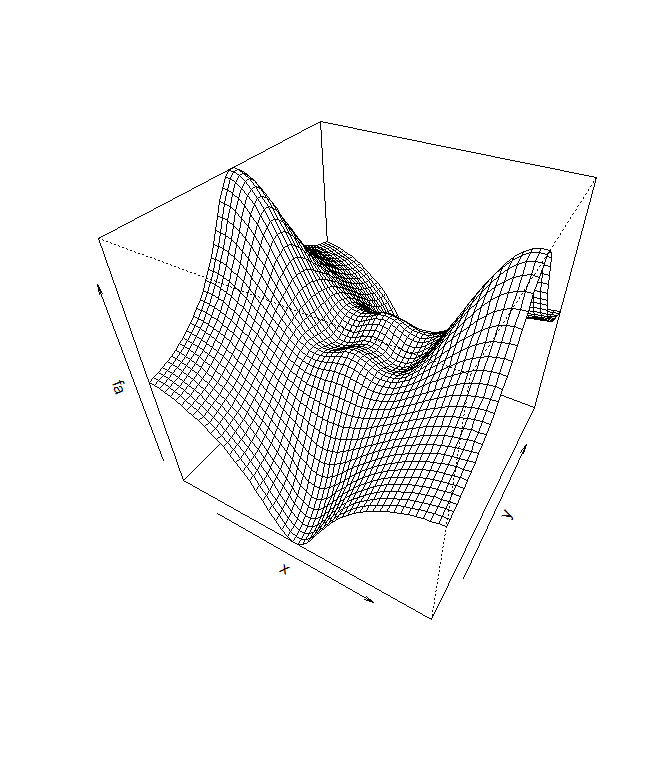
The image() function works the same way as contour(), except that it produces a color-coded plot whose colors depend on the z value. This is known as a heatmap, and is sometimes used to plot temperature in weather heatmap forecasts. Alternatively, persp() can be used to produce a three-dimensional plot. The arguments theta and phi control the angles at which the plot is viewed.

persp(x,y,fa)

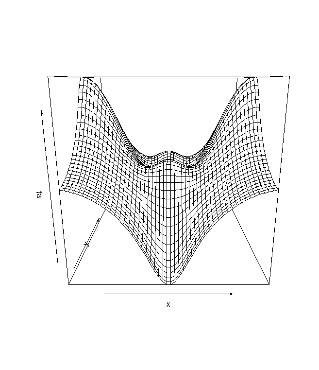
persp(x,y,fa ,theta =30, phi =40)

persp(x,y,fa ,theta =30, phi =70)