# Introduction to TensorFlow for Artificial Intelligence, Machine Learning, and Deep Learning
# A New Programming Paradigm
# A primer in machine learning
We can represent that with this diagram. Rules and data go in answers come out. Rules are expressed in a programming language and data can come from a variety of sources from local variables all the way up to databases. Machine learning rearranges this diagram where we put answers in data in and then we get rules out.
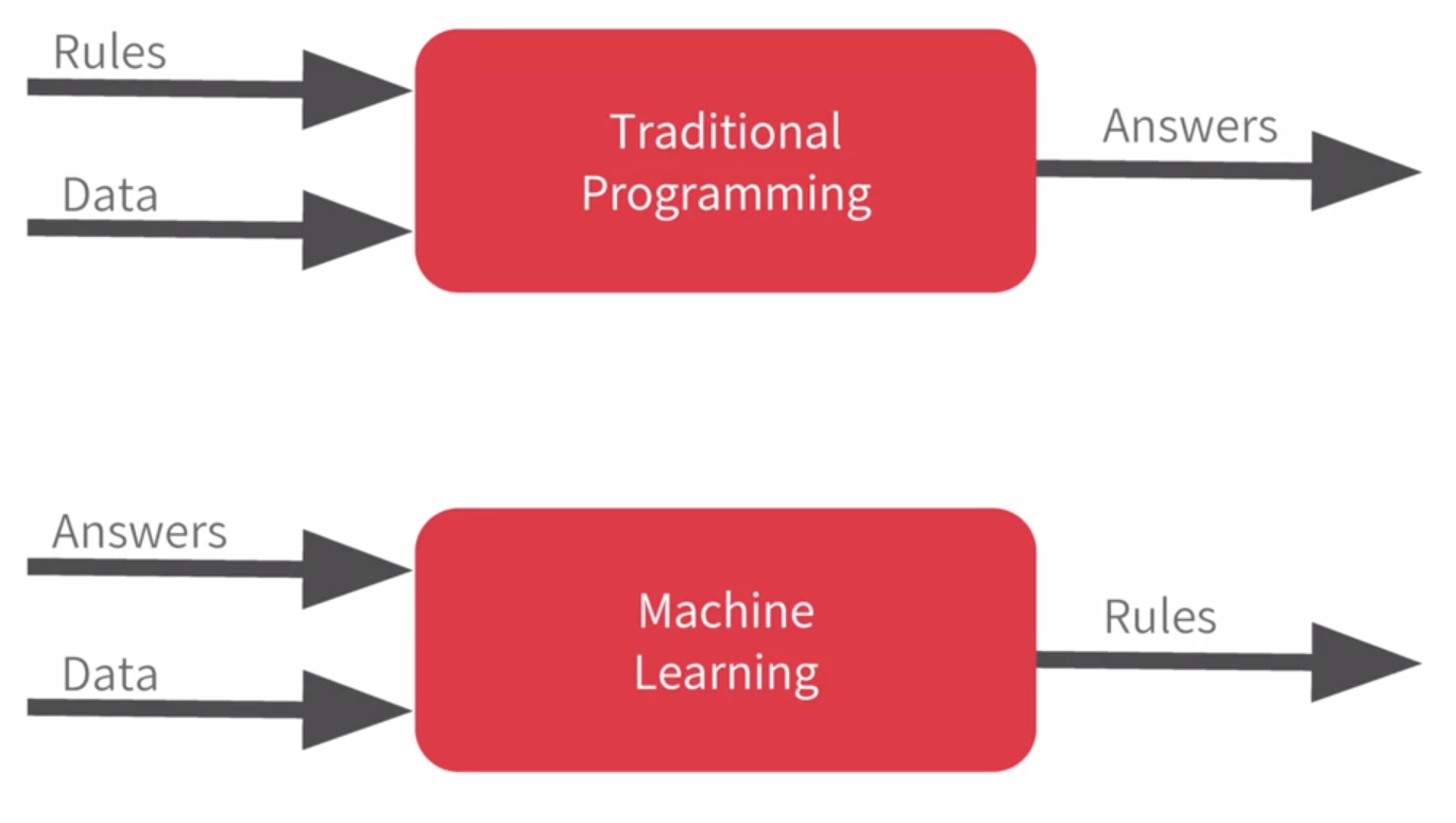
So instead of us as developers figuring out the rules when should the brick be removed, when should the player's life end, or what's the desired analytic for any other concept, what we will do is we can get a bunch of examples for what we want to see and then have the computer figure out the rules. Now, this is particularly valuable for problems that you can't solve by figuring the rules out for yourself.
So consider this example, activity recognition. If I'm building a device that detects if somebody is say walking and I have data about their speed, I might write code like this and if they're running well that's a faster speed so I could adapt my code to this and if they're biking, well that's not too bad either. I can adapt my code like this. But then I have to do golf recognition too, now my concept becomes broken.
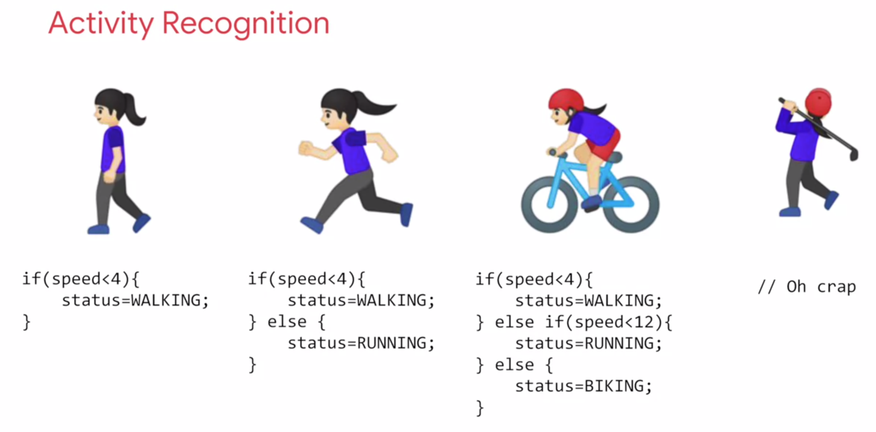
But not only that, doing it by speed alone of course is quite naive. We walk and run at different speeds uphill and downhill and other people walk and run at different speeds to us. So, let's go back to the diagram. Ultimately machine learning is very similar but we're just flipping the axes.
So, instead of me trying to express the problem as rules when often that isn't even possible, I'll have to compromise.
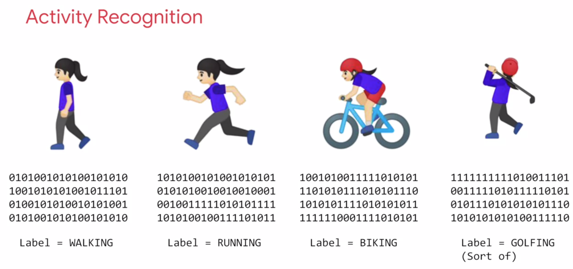
The new paradigm is that I get lots and lots of examples and then I have labels on those examples and I use the data to say this is what walking looks like, this is what running looks like, this is what biking looks like and yes, even this is what golfing looks like.
So, then it becomes answers and data in with rules being inferred by the machine. A machine learning algorithm then figures out the specific patterns in each set of data that determines the distinctiveness of each.
That's what's so powerful and exciting about this programming paradigm. It's more than just a new way of doing the same old thing. It opens up new possibilities that were infeasible to do before.
# The ‘Hello World’ of neural networks
Earlier, we mentioned that machine learning is all about a computer learning the patterns that distinguish things. Like for activity recognition, it was the pattern of walking, running and biking that can be learned from various sensors on a device.
To show how that works, let's take a look at a set of numbers and see if you can determine the pattern between them.
X = -1, 0, 1, 2, 3, 4
Y = -3, -1, 1, 3, 5, 7
2
Y = (X*2)-1
Congratulations, you've just done the basics of machine learning in your head. So let's take a look at it in code now.
Okay, here's our first line of code.
model = tf.keras.Sequential([tf.keras.layers.Dense(units=1, input_shape=[1])])
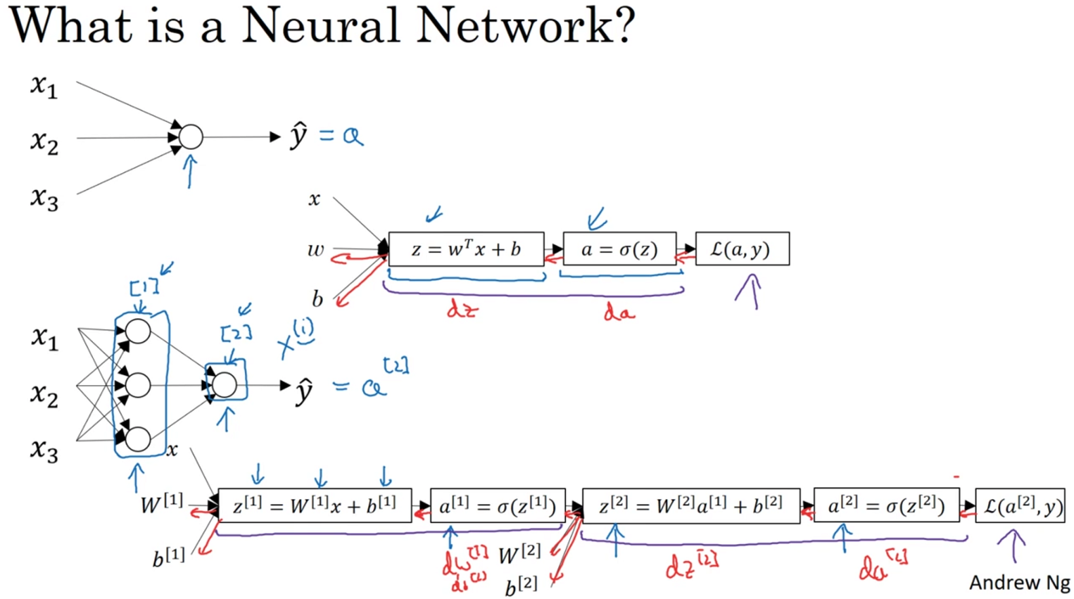
This is written using Python and TensorFlow and an API in TensorFlow called keras. Keras makes it really easy to define neural networks. A neural network is basically a set of functions which can learn patterns. Don't worry if there were a lot of new concepts here. They will become clear quite quickly as you work through them. The simplest possible neural network is one that has only one neuron in it, and that's what this line of code does.
In keras, you use the word dense to define a layer of connected neurons. There's only one dense here. So there's only one layer and there's only one unit in it, so it's a single neuron. Successive layers are defined in sequence, hence the word sequential. But as I've said, there's only one. So you have a single neuron.
You define the shape of what's input to the neural network in the first, and in this case the only layer, and you can see that our input shape is super simple. It's just one value.
You've probably seen that for machine learning, you need to know and use a lot of math, calculus probability and the like. It's really good to understand that as you want to optimize your models but the nice thing for now about TensorFlow and keras is that a lot of that math is implemented for you in functions. There are two function roles that you should be aware of though and these are loss functions and optimizers. This code defines them.
model.compile(optimizer='sgd', loss='mean_squared_error')
I like to think about it this way. The neural network has no idea of the relationship between X and Y, so it makes a guess. Say it guesses Y equals 10X minus 10. It will then use the data that it knows about, that's the set of Xs and Ys that we've already seen to measure how good or how bad its guess was. The loss function measures this and then gives the data to the optimizer which figures out the next guess. So the optimizer thinks about how good or how badly the guess was done using the data from the loss function. Then the logic is that each guess should be better than the one before. As the guesses get better and better, an accuracy approaches 100 percent, the term convergence is used.
Our next step is to represent the known data. These are the Xs and the Ys that you saw earlier. The np.array is using a Python library called numpy that makes data representation particularly enlists much easier. So here you can see we have one list for the Xs and another one for the Ys.
xs = np.array([-1.0, 0.0, 1.0, 2.0, 3.0, 4.0], dtype=float)
ys = np.array([-3.0, -1.0, 1.0, 3.0, 5.0, 7.0], dtype=float)
2
The training takes place in the fit command. Here we're asking the model to figure out how to fit the X values to the Y values. The epochs equals 500 value means that it will go through the training loop 500 times. This training loop is what we described earlier. Make a guess, measure how good or how bad the guesses with the loss function, then use the optimizer and the data to make another guess and repeat this.
model.fit(xs, ys, epochs=500)
When the model has finished training, it will then give you back values using the predict method. So it hasn't previously seen 10, and what do you think it will return when you pass it a 10?
Epoch 1/500
1/1 [==============================] - 0s 0s/step - loss: 15.6188
Epoch 2/500
1/1 [==============================] - 0s 0s/step - loss: 12.5317
Epoch 3/500
1/1 [==============================] - 0s 0s/step - loss: 10.0979
.
.
.
Epoch 497/500
1/1 [==============================] - 0s 0s/step - loss: 4.2759e-05
Epoch 498/500
1/1 [==============================] - 0s 0s/step - loss: 4.1881e-05
Epoch 499/500
1/1 [==============================] - 0s 0s/step - loss: 4.1020e-05
Epoch 500/500
1/1 [==============================] - 0s 0s/step - loss: 4.0177e-05
[[18.981508]]
2
3
4
5
6
7
8
9
10
11
12
13
14
15
16
17
18
Now you might think it would return 19 because after all Y equals 2X minus 1, and you think it should be 19. But when you try this in the workbook yourself, you'll see that it will return a value very close to 19 but not exactly 19. Now why do you think that would be?
Ultimately there are two main reasons. The first is that you trained it using very little data. There's only six points. Those six points are linear but there's no guarantee that for every X, the relationship will be Y equals 2X minus 1. There's a very high probability that Y equals 19 for X equals 10, but the neural network isn't positive. So it will figure out a realistic value for Y. That's the second main reason. When using neural networks, as they try to figure out the answers for everything, they deal in probability. You'll see that a lot and you'll have to adjust how you handle answers to fit. Keep that in mind as you work through the code.
Here is the full code:
import tensorflow as tf
import numpy as np


model = tf.keras.Sequential([tf.keras.layers.Dense(units=1, input_shape=[1])])

model.compile(optimizer='sgd', loss='mean_squared_error')

xs = np.array([-1.0, 0.0, 1.0, 2.0, 3.0, 4.0], dtype=float)
ys = np.array([-3.0, -1.0, 1.0, 3.0, 5.0, 7.0], dtype=float)

model.fit(xs, ys, epochs=500)

print(model.predict([10.0]))
2
3
4
5
6
7
8
9
10
11
12
13
14
Or, we can import keras from tensorflow and ru like this:
import numpy as np
from tensorflow import keras

model = keras.Sequential([keras.layers.Dense(units=1, input_shape=[1])])

model.compile(optimizer='sgd', loss='mean_squared_error')

xs = np.array([-1.0, 0.0, 1.0, 2.0, 3.0, 4.0], dtype=float)
ys = np.array([-3.0, -1.0, 1.0, 3.0, 5.0, 7.0], dtype=float)

model.fit(xs, ys, epochs=500)

print(model.predict([10.0]))
2
3
4
5
6
7
8
9
10
11
12
13
# Adding TensorBoard
import tensorflow as tf
import numpy as np

import time
from tensorflow.keras.callbacks import TensorBoard

NAME = "LinearRegression-{}".format(int(time.time()))
tensorboard = TensorBoard(log_dir='logs/{}'.format(NAME))

model = tf.keras.Sequential([tf.keras.layers.Dense(units=1, input_shape=[1])])

model.compile(optimizer='sgd', loss='mean_squared_error')

xs = np.array([-1.0, 0.0, 1.0, 2.0, 3.0, 4.0], dtype=float)
ys = np.array([-3.0, -1.0, 1.0, 3.0, 5.0, 7.0], dtype=float)

model.fit(xs, ys, epochs=500, callbacks=[tensorboard])

print(model.predict([10.0]))
2
3
4
5
6
7
8
9
10
11
12
13
14
15
16
17
18
19

# Introduction to Computer Vision
Let's now take this to the next level by solving a real problem, computer vision. Computer vision is the field of having a computer understand and label what is present in an image.
Consider this slide. When you look at it, you can interpret what a shirt is or what a shoe is, but how would you program for that? If an extra terrestrial who had never seen clothing walked into the room with you, how would you explain the shoes to him? It's really difficult, if not impossible to do right? And it's the same problem with computer vision.
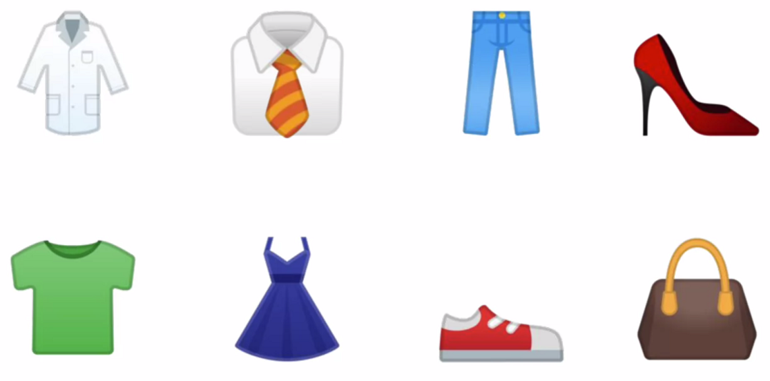
So, one way to solve that is to use lots of pictures of clothing and tell the computer what that's a picture of and then have the computer figure out the patterns that give you the difference between a shoe, and a shirt, and a handbag, and a coat. That's what you're going to learn how to do in this section.
Fortunately, there's a data set called Fashion MNIST which gives a 70 thousand images spread across 10 different items of clothing. These images have been scaled down to 28 by 28 pixels. Now usually, the smaller the better because the computer has less processing to do. But of course, you need to retain enough information to be sure that the features and the object can still be distinguished. If you look at this slide you can still tell the difference between shirts, shoes, and handbags. So this size does seem to be ideal, and it makes it great for training a neural network.
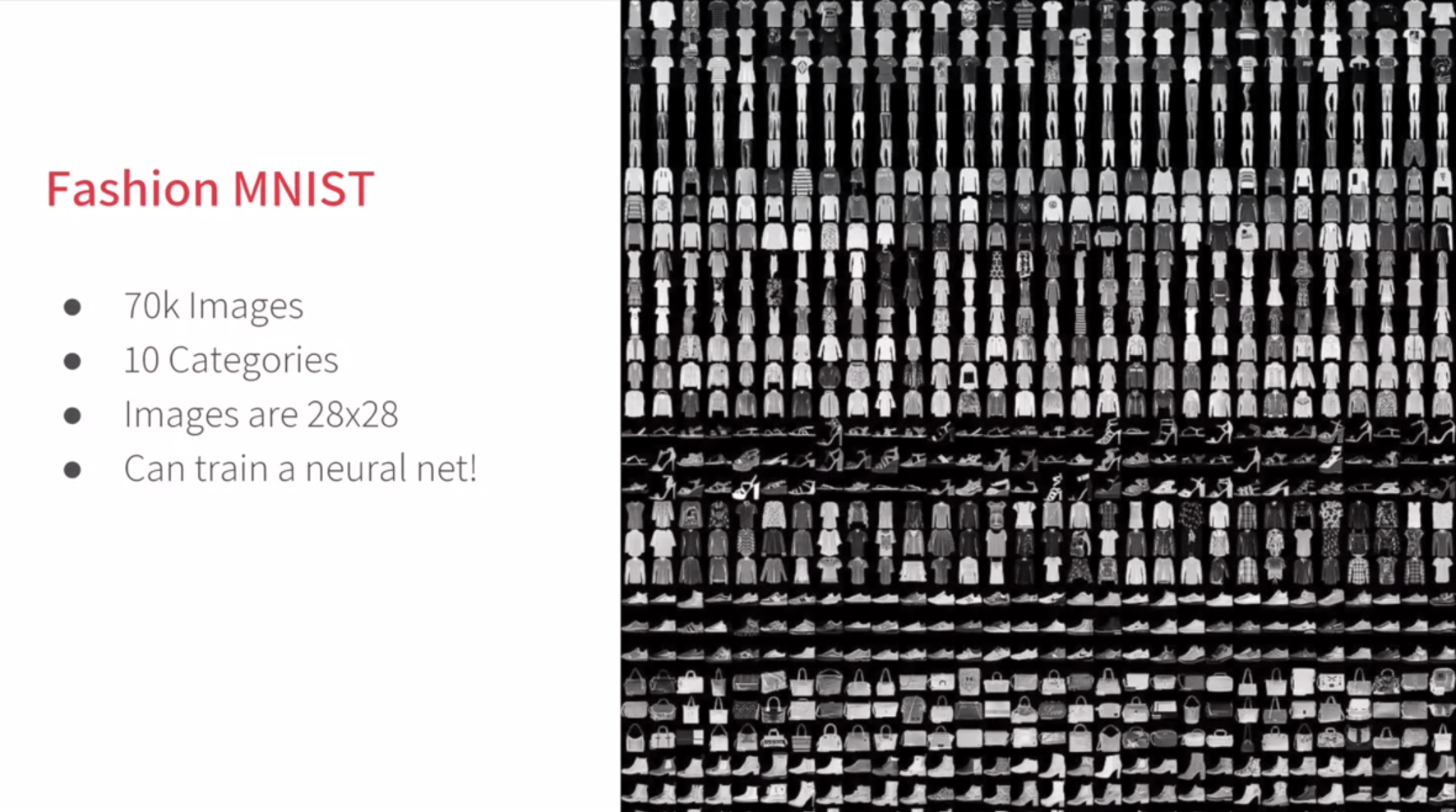
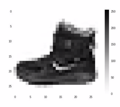
The images are also in gray scale, so the amount of information is also reduced. Each pixel can be represented in values from zero to 255 and so it's only one byte per pixel. With 28 by 28 pixels in an image, only 784 bytes are needed to store the entire image. Despite that, we can still see what's in the image and in this case, it's an ankle boot, right?
# Writing code to load training data
So, what will handling this look like in code? In the previous lesson, you learned about TensorFlow and Keras, and how to define a super simple neural network with them.
In this lesson, you're going to use them to go a little deeper but the overall API should look familiar.
The one big difference will be in the data. The last time you had your six pairs of numbers, so you could hard code it. This time you have to load 70,000 images off the disk, so there'll be a bit of code to handle that. Fortunately, it's still quite simple because Fashion-MNIST is available as a data set with an API call in TensorFlow. We simply declare an object of type MNIST loading it from the Keras database.
import tensorflow as tf
import numpy as np

from tensorflow import keras

fashion_mnist = keras.datasets.fashion_mnist
2
3
4
5
6
On this object, if we call the load data method, it will return four lists to us. That's the training data, the training labels, the testing data, and the testing labels.
(train_images, train_labels), (test_images, test_labels) = fashion_mnist.load_data()
Now, what are these you might ask? Well, when building a neural network like this, it's a nice strategy to use some of your data to train the neural network and similar data that the model hasn't yet seen to test how good it is at recognizing the images. So in the Fashion-MNIST data set, 60,000 of the 70,000 images are used to train the network, and then 10,000 images, one that it hasn't previously seen, can be used to test just how good or how bad it is performing.
So this code will give you those sets. Then, each set has data, the images themselves and labels and that's what the image is actually of.
So for example, the training data will contain images like this one, and a label that describes the image like this. While this image is an ankle boot, the label describing it is the number nine. Now, why do you think that might be?
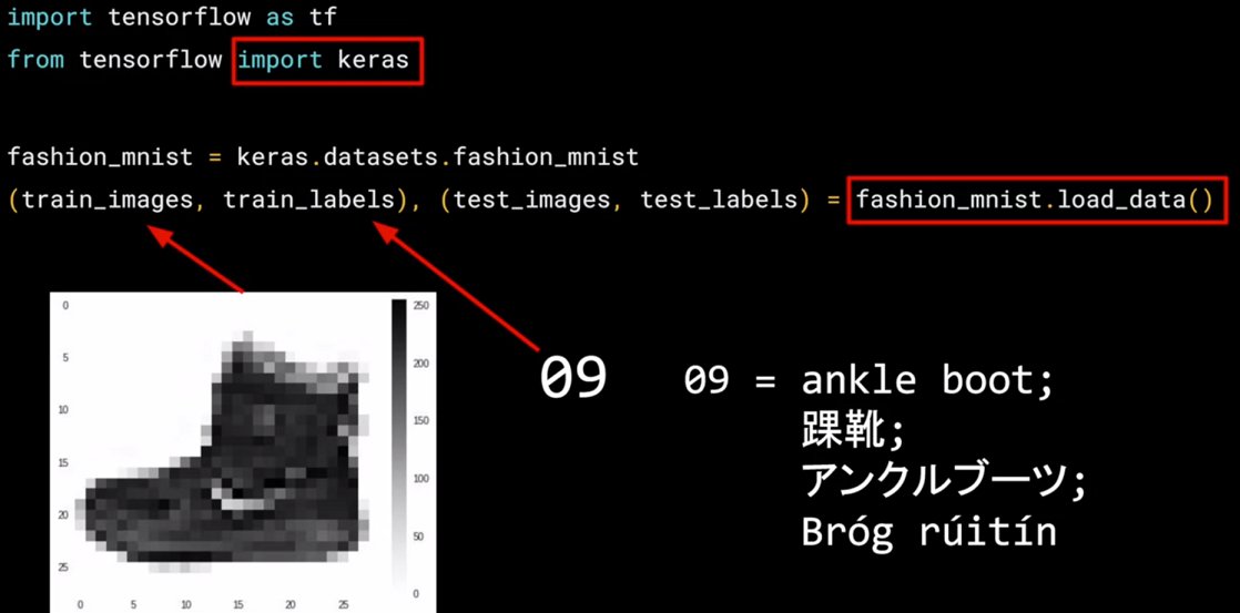
There's two main reasons. First, of course, is that computers do better with numbers than they do with texts. Second, importantly, is that this is something that can help us reduce bias. If we labeled it as an ankle boot, we would be of course biasing towards English speakers. But with it being a numeric label, we can then refer to it in our appropriate language be it English, Chinese, Japanese, or here, even Irish Gaelic.
# Coding a Computer Vision Neural Network
Okay. So now we will look at the code for the neural network definition. Remember last time we had a sequential with just one layer in it. Now we have three layers.
model = keras.Sequential([
    keras.layers.Flatten(input_shape[28, 28]),
    keras.layers.Dense(128, activation='relu'),
    keras.layers.Dense(10, activation='softmax')
])
2
3
4
5
The important things to look at are the first and the last layers.
The last layer has 10 neurons in it because we have ten classes of clothing in the dataset. They should always match.
The first layer is a flatten layer with the input shaping 28 by 28. Now, if you remember our images are 28 by 28, so we're specifying that this is the shape that we should expect the data to be in. Flatten takes this 28 by 28 square and turns it into a simple linear array.
The interesting stuff happens in the middle layer, sometimes also called a hidden layer. This is a 128 neurons in it, and I'd like you to think about these as variables in a function. Maybe call them x1, x2 x3, etc. Now, there exists a rule that incorporates all of these that turns the 784 values of an ankle boot into the value nine, and similar for all of the other 70,000. It's too complex a function for you to see by mapping the images yourself, but that's what a neural net does.
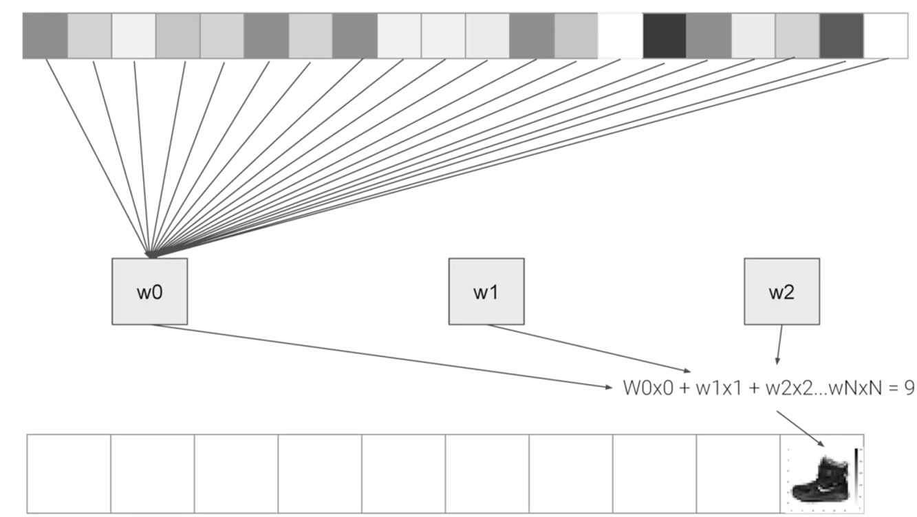
So, for example, if you then say the function was y equals w1 times x1, plus w2 times x2, plus w3 times x3, all the way up to a w128 times x128. By figuring out the values of w, then y will be nine, when you have the input value of the shoe. You'll see that it's doing something very, very similar to what we did earlier when we figured out y equals 2x minus one. In that case the two, was the weight of x. So, I'm saying y equals w1 times x1, etc. Now, don't worry if this isn't very clear right now. Over time, you will get the hang of it, seeing that it works, and there's also some tools that will allow you to peek inside to see what's going on. The important thing for now is to get the code working, so you can see a classification scenario for yourself. You can also tune the neural network by adding, removing and changing layer size to see the impact.
# Walk through a Notebook for computer vision
So you just saw how to create a neural network that gives basic computer vision capabilities to recognize different items of clothing. Let's now work through a workbook that has all of the code to do that. You'll then go through this workbook yourself and if you want you can try some exercises. Let's start by importing TensorFlow. I'm going to get the fashion MNIST data using tf.kares.datasets. By calling the load data method, I get training data and labels as well as test data and labels.
#%%
import tensorflow as tf
print(tf.__version__)
import numpy as np

from tensorflow import keras


#%%
mnist = keras.datasets.fashion_mnist


#%%
(train_images, train_labels), (test_images, test_labels) = mnist.load_data()
2
3
4
5
6
7
8
9
10
11
12
13
14
The data for a particular image is a grid of values from zero to 255 with pixel Grayscale values. Using matplotlib, I can plot these as an image to make it easier to inspect. I can also print out the raw values so we can see what they look like. Here you can see the raw values for the pixel numbers from zero to 255, and here you can see the actual image. That was for the first image in the array.
#%%
import matplotlib.pyplot as plt
plt.imshow(train_images[0])
print(train_labels[0])
print(train_images[0])
2
3
4
5
9
[[  0   0   0   0   0   0   0   0   0   0   0   0   0   0   0   0   0   0
    0   0   0   0   0   0   0   0   0   0]
 [  0   0   0   0   0   0   0   0   0   0   0   0   0   0   0   0   0   0
    0   0   0   0   0   0   0   0   0   0]
 [  0   0   0   0   0   0   0   0   0   0   0   0   0   0   0   0   0   0
    0   0   0   0   0   0   0   0   0   0]
 [  0   0   0   0   0   0   0   0   0   0   0   0   1   0   0  13  73   0
    0   1   4   0   0   0   0   1   1   0]
 [  0   0   0   0   0   0   0   0   0   0   0   0   3   0  36 136 127  62
   54   0   0   0   1   3   4   0   0   3]
 [  0   0   0   0   0   0   0   0   0   0   0   0   6   0 102 204 176 134
  144 123  23   0   0   0   0  12  10   0]
 [  0   0   0   0   0   0   0   0   0   0   0   0   0   0 155 236 207 178
  107 156 161 109  64  23  77 130  72  15]
 [  0   0   0   0   0   0   0   0   0   0   0   1   0  69 207 223 218 216
  216 163 127 121 122 146 141  88 172  66]
 [  0   0   0   0   0   0   0   0   0   1   1   1   0 200 232 232 233 229
  223 223 215 213 164 127 123 196 229   0]
 [  0   0   0   0   0   0   0   0   0   0   0   0   0 183 225 216 223 228
  235 227 224 222 224 221 223 245 173   0]
 [  0   0   0   0   0   0   0   0   0   0   0   0   0 193 228 218 213 198
  180 212 210 211 213 223 220 243 202   0]
 [  0   0   0   0   0   0   0   0   0   1   3   0  12 219 220 212 218 192
  169 227 208 218 224 212 226 197 209  52]
 [  0   0   0   0   0   0   0   0   0   0   6   0  99 244 222 220 218 203
  198 221 215 213 222 220 245 119 167  56]
 [  0   0   0   0   0   0   0   0   0   4   0   0  55 236 228 230 228 240
  232 213 218 223 234 217 217 209  92   0]
 [  0   0   1   4   6   7   2   0   0   0   0   0 237 226 217 223 222 219
  222 221 216 223 229 215 218 255  77   0]
 [  0   3   0   0   0   0   0   0   0  62 145 204 228 207 213 221 218 208
  211 218 224 223 219 215 224 244 159   0]
 [  0   0   0   0  18  44  82 107 189 228 220 222 217 226 200 205 211 230
  224 234 176 188 250 248 233 238 215   0]
 [  0  57 187 208 224 221 224 208 204 214 208 209 200 159 245 193 206 223
  255 255 221 234 221 211 220 232 246   0]
 [  3 202 228 224 221 211 211 214 205 205 205 220 240  80 150 255 229 221
  188 154 191 210 204 209 222 228 225   0]
 [ 98 233 198 210 222 229 229 234 249 220 194 215 217 241  65  73 106 117
  168 219 221 215 217 223 223 224 229  29]
 [ 75 204 212 204 193 205 211 225 216 185 197 206 198 213 240 195 227 245
  239 223 218 212 209 222 220 221 230  67]
 [ 48 203 183 194 213 197 185 190 194 192 202 214 219 221 220 236 225 216
  199 206 186 181 177 172 181 205 206 115]
 [  0 122 219 193 179 171 183 196 204 210 213 207 211 210 200 196 194 191
  195 191 198 192 176 156 167 177 210  92]
 [  0   0  74 189 212 191 175 172 175 181 185 188 189 188 193 198 204 209
  210 210 211 188 188 194 192 216 170   0]
 [  2   0   0   0  66 200 222 237 239 242 246 243 244 221 220 193 191 179
  182 182 181 176 166 168  99  58   0   0]
 [  0   0   0   0   0   0   0  40  61  44  72  41  35   0   0   0   0   0
    0   0   0   0   0   0   0   0   0   0]
 [  0   0   0   0   0   0   0   0   0   0   0   0   0   0   0   0   0   0
    0   0   0   0   0   0   0   0   0   0]
 [  0   0   0   0   0   0   0   0   0   0   0   0   0   0   0   0   0   0
    0   0   0   0   0   0   0   0   0   0]]
2
3
4
5
6
7
8
9
10
11
12
13
14
15
16
17
18
19
20
21
22
23
24
25
26
27
28
29
30
31
32
33
34
35
36
37
38
39
40
41
42
43
44
45
46
47
48
49
50
51
52
53
54
55
56
57
Let's take a look at the image at index 42 instead, and we can see the different pixel values and the actual graphic.
plt.imshow(train_images[42])
print(train_labels[42])
print(train_images[42])
2
3
9
[[  0   0   0   0   0   0   0   0   0   0   0   0   0   0   0   0   0   0
    0   0   0   0   0   0   0   0   0   0]
 [  0   0   0   0   0   0   0   0   0   0   0   0   0   0   0   0   0   0
    0   0   0   0   0   0   0   0   0   0]
 [  0   0   0   0   0   0   0   0   0   0   0   0   0   0   0   0   0   0
    0   0   0   0   0   0   0   0   0   0]
 [  0   0   0   0   0   0   0   0   0   0   0   0   0   0   0   0   0   0
    0   0   0   0   0   0   0   0   0   0]
 [  0   0   0   0   0   0   0   0   0   0   0   0   0   0   0   0   0   0
    0   0   0   0   0   0   0   0   0   0]
 [  0   0   0   0   0   0   0   0   0   0   0   0   0   0   0   0  82 187
   26   0   0   0   0   0   0   0   0   0]
 [  0   0   0   0   0   0   0   0   0   1   0   0   1   0   0 179 240 237
  255 240 139  83  64  43  60  54   0   1]
 [  0   0   0   0   0   0   0   0   0   1   0   0   1   0  58 239 222 234
  238 246 252 254 255 248 255 187   0   0]
 [  0   0   0   0   0   0   0   0   0   0   2   3   0   0 194 239 226 237
  235 232 230 234 234 233 249 171   0   0]
 [  0   0   0   0   0   0   0   0   0   1   1   0   0  10 255 226 242 239
  238 239 240 239 242 238 248 192   0   0]
 [  0   0   0   0   0   0   0   0   0   0   0   0   0 172 245 229 240 241
  240 241 243 243 241 227 250 209   0   0]
 [  0   0   0   0   0   0   0   0   0   6   5   0  62 255 230 236 239 241
  242 241 242 242 238 238 242 253   0   0]
 [  0   0   0   0   0   0   0   0   0   3   0   0 255 235 228 244 241 241
  244 243 243 244 243 239 235 255  22   0]
 [  0   0   0   0   0   0   0   0   0   0   0 246 228 220 245 243 237 241
  242 242 242 243 239 237 235 253 106   0]
 [  0   0   3   4   4   2   1   0   0  18 243 228 231 241 243 237 238 242
  241 240 240 240 235 237 236 246 234   0]
 [  1   0   0   0   0   0   0   0  22 255 238 227 238 239 237 241 241 237
  236 238 239 239 239 239 239 237 255   0]
 [  0   0   0   0   0  25  83 168 255 225 225 235 228 230 227 225 227 231
  232 237 240 236 238 239 239 235 251  62]
 [  0 165 225 220 224 255 255 233 229 223 227 228 231 232 235 237 233 230
  228 230 233 232 235 233 234 235 255  58]
 [ 52 251 221 226 227 225 225 225 226 226 225 227 231 229 232 239 245 250
  251 252 254 254 252 254 252 235 255   0]
 [ 31 208 230 233 233 237 236 236 241 235 241 247 251 254 242 236 233 227
  219 202 193 189 186 181 171 165 190  42]
 [ 77 199 172 188 199 202 218 219 220 229 234 222 213 209 207 210 203 184
  152 171 165 162 162 167 168 157 192  78]
 [  0  45 101 140 159 174 182 186 185 188 195 197 188 175 133  70  19   0
    0 209 231 218 222 224 227 217 229  93]
 [  0   0   0   0   0   0   2  24  37  45  32  18  11   0   0   0   0   0
    0  72  51  53  37  34  29  31   5   0]
 [  0   0   0   0   0   0   0   0   0   0   0   0   0   0   0   0   0   0
    0   0   0   0   0   0   0   0   0   0]
 [  0   0   0   0   0   0   0   0   0   0   0   0   0   0   0   0   0   0
    0   0   0   0   0   0   0   0   0   0]
 [  0   0   0   0   0   0   0   0   0   0   0   0   0   0   0   0   0   0
    0   0   0   0   0   0   0   0   0   0]
 [  0   0   0   0   0   0   0   0   0   0   0   0   0   0   0   0   0   0
    0   0   0   0   0   0   0   0   0   0]
 [  0   0   0   0   0   0   0   0   0   0   0   0   0   0   0   0   0   0
    0   0   0   0   0   0   0   0   0   0]]
2
3
4
5
6
7
8
9
10
11
12
13
14
15
16
17
18
19
20
21
22
23
24
25
26
27
28
29
30
31
32
33
34
35
36
37
38
39
40
41
42
43
44
45
46
47
48
49
50
51
52
53
54
55
56
57
58
Our image has values from 0 to 255, but neural networks work better with normalized data. So, let's change it to between zero and one simply by dividing every value by 255. In Python, you can actually divide an entire array with one line of code like this.
training_images = training_images / 255.0
test_images = test_images / 255.0
2
So now we design our model. As explained earlier, there's an input layer in the shape of the data and an output layer in the shape of the classes, and one hidden layer that tries to figure out the roles between them.
model = keras.Sequential([
    keras.layers.Flatten(),
    keras.layers.Dense(128, activation='relu'),
    keras.layers.Dense(10, activation='softmax')
])
2
3
4
5
Now we compile the model to finding the loss function and the optimizer, and the goal of these is as before, to make a guess as to what the relationship is between the input data and the output data, measure how well or how badly it did using the loss function, use the optimizer to generate a new guess and repeat.
We can then try to fit the training images to the training labels. We'll just do it for five epochs to be quick.
model.compile(optimizer='adam',
              loss='sparse_categorical_crossentropy')

model.fit(training_images, training_labels, epochs=5)
2
3
4
Epoch 1/5
1875/1875 [==============================] - 1s 655us/step - loss: 0.4961
Epoch 2/5
1875/1875 [==============================] - 1s 619us/step - loss: 0.3749
Epoch 3/5
1875/1875 [==============================] - 1s 621us/step - loss: 0.3349
Epoch 4/5
1875/1875 [==============================] - 1s 628us/step - loss: 0.3098
Epoch 5/5
1875/1875 [==============================] - 1s 646us/step - loss: 0.2923
2
3
4
5
6
7
8
9
10
We spend about 5 seconds training it over five epochs and we end up with a loss of about 0.29. That means it's pretty accurate in guessing the relationship between the images and their labels. That's not great, but considering it was done in just 5 seconds with a very basic neural network, it's not bad either.
But a better measure of performance can be seen by trying the test data. These are images that the network has not yet seen. You would expect performance to be worse, but if it's much worse, you have a problem. As you can see, it's about 0.3505 loss, meaning it's a little bit less accurate on the test set. It's not great either, but we know we're doing something right.
model.evaluate(test_images, test_labels)
  1/313 [..............................] - ETA: 0s - loss: 0.3092
313/313 [==============================] - 0s 492us/step - loss: 0.3505
0.3505074679851532
2
3
# Using TensorBoard
#%%
import tensorflow as tf
print(tf.__version__)
import numpy as np

from tensorflow import keras

import time
from tensorflow.keras.callbacks import TensorBoard

NAME = "FashionMNIST-{}".format(int(time.time()))
tensorboard = TensorBoard(log_dir='logs/{}'.format(NAME))

#%%
mnist = keras.datasets.fashion_mnist


#%%
(training_images, training_labels), (test_images, test_labels) = mnist.load_data()


#%%
import matplotlib.pyplot as plt
plt.imshow(training_images[42])
print(training_labels[42])
print(training_images[42])

#%%

training_images = training_images / 255.0
test_images = test_images / 255.0


#%%
model = keras.Sequential([
    keras.layers.Flatten(),
    keras.layers.Dense(128, activation='relu'),
    keras.layers.Dense(10, activation='softmax')
])

#%%

model.compile(optimizer='adam',
              loss='sparse_categorical_crossentropy')

model.fit(training_images, training_labels, epochs=5, callbacks=[tensorboard])


#%%

model.evaluate(test_images, test_labels)
2
3
4
5
6
7
8
9
10
11
12
13
14
15
16
17
18
19
20
21
22
23
24
25
26
27
28
29
30
31
32
33
34
35
36
37
38
39
40
41
42
43
44
45
46
47
48
49
50
51

Your job now is to go through the workbook, try the exercises and see by tweaking the parameters on the neural network or changing the epochs, if there's a way for you to get it above 0.71 loss accuracy on training data and 0.66 accuracy on test data, give it a try for yourself.
WARNING
Try the exercises once you have access to the notebook.
After including another layer with 'tanh' and increasing the epoch number to 100 we got:
Epoch 1/100
   1/1875 [..............................] - ETA: 0s - loss: 2.3306
1875/1875 [==============================] - 2s 987us/step - loss: 0.4647
Epoch 2/100
1875/1875 [==============================] - 2s 807us/step - loss: 0.3577
Epoch 3/100
1875/1875 [==============================] - 1s 778us/step - loss: 0.3204
Epoch 4/100
1875/1875 [==============================] - 1s 753us/step - loss: 0.2969
Epoch 5/100
1875/1875 [==============================] - 1s 759us/step - loss: 0.2824
.
.
.
Epoch 97/100
1875/1875 [==============================] - 1s 793us/step - loss: 0.0645
Epoch 98/100
1875/1875 [==============================] - 2s 815us/step - loss: 0.0602
Epoch 99/100
1875/1875 [==============================] - 2s 821us/step - loss: 0.0604
Epoch 100/100
1875/1875 [==============================] - 2s 815us/step - loss: 0.0601
2
3
4
5
6
7
8
9
10
11
12
13
14
15
16
17
18
19
20
21
22

#%%
import tensorflow as tf
print(tf.__version__)
import numpy as np

from tensorflow import keras

import time
from tensorflow.keras.callbacks import TensorBoard

NAME = "FashionMNIST-100Epochs-2Layers_EarlyStopping-{}".format(int(time.time()))
tensorboard = TensorBoard(log_dir='logs/{}'.format(NAME))

#%%
mnist = keras.datasets.fashion_mnist


#%%
(training_images, training_labels), (test_images, test_labels) = mnist.load_data()


#%%
import matplotlib.pyplot as plt
plt.imshow(training_images[42])
print(training_labels[42])
print(training_images[42])

#%%

training_images = training_images / 255.0
test_images = test_images / 255.0


#%%
model = keras.Sequential([
    keras.layers.Flatten(),
    keras.layers.Dense(128, activation='relu'),
    keras.layers.Dense(128, activation='tanh'),
    keras.layers.Dense(10, activation='softmax')
])

#%%

model.compile(optimizer='adam',
              loss='sparse_categorical_crossentropy')

model.fit(training_images, training_labels, epochs=100, callbacks=[tensorboard], verbose=2)


#%%

model.evaluate(test_images, test_labels)
2
3
4
5
6
7
8
9
10
11
12
13
14
15
16
17
18
19
20
21
22
23
24
25
26
27
28
29
30
31
32
33
34
35
36
37
38
39
40
41
42
43
44
45
46
47
48
49
50
51
52
# Using Callbacks to control training
A question I often get at this point from programmers in particular when experimenting with different numbers of epochs is, How can I stop training when I reach a point that I want to be at? What do I always have to hard code it to go for certain number of epochs?
Well, the good news is that, the training loop does support callbacks. So in every epoch, you can callback to a code function, having checked the metrics. If they're what you want to say, then you can cancel the training at that point.
Let's take a look. Okay, so here's our code for training the neural network to recognize the fashion images. In particular, keep an eye on the model.fit function that executes the training loop. You can see that here.
mnist = keras.datasets.fashion_mnist
(training_images, training_labels), (test_images, test_labels) = mnist.load_data()
training_images = training_images / 255.0
test_images = test_images / 255.0

model = keras.models.Sequential([
    keras.layers.Flatten(),
    keras.layers.Dense(512, activation='relu'),
    keras.layers.Dense(10, activation='softmax')
])

model.compile(optimizer='adam',
              loss='sparse_categorical_crossentropy')

model.fit(training_images, training_labels, epochs=5)
2
3
4
5
6
7
8
9
10
11
12
13
14
15
What we'll now do is write a callback in Python. Here's the code. It's implemented as a separate class, but that can be in-line with your other code. It doesn't need to be in a separate file.
class MyCallback(keras.callbacks.Callback):
    def on_epoch_end(self, epoch, logs={}):
        if logs.get('loss') < 0.4:
            print("\nLoss is low so cancelling training!")
            self.model.stop_training = True
2
3
4
5
In it, we'll implement the on_epoch_end function, which gets called by the callback whenever the epoch ends. It also sends a logs object which contains lots of great information about the current state of training. For example, the current loss is available in the logs, so we can query it for certain amount. For example, here I'm checking if the loss is less than 0.4 and canceling the training itself. Now that we have our callback, let's return to the rest of the code, and there are two modifications that we need to make.
First, we instantiate the class that we just created, we do that with this code. Then, in my model.fit, I used the callbacks parameter and pass it this instance of the class. Let's see this in action.
import tensorflow as tf
from tensorflow import keras

class MyCallback(keras.callbacks.Callback):
    def on_epoch_end(self, epoch, logs={}):
        if logs.get('loss') < 0.4:
            print("\nLoss is low so cancelling training!")
            self.model.stop_training = True
callbacks = MyCallback()

mnist = keras.datasets.fashion_mnist

(training_images, training_labels), (test_images, test_labels) = mnist.load_data()

training_images = training_images / 255.0
test_images = test_images / 255.0

model = keras.models.Sequential([
    keras.layers.Flatten(),
    keras.layers.Dense(128, activation='relu'),
    keras.layers.Dense(128, activation='tanh'),
    keras.layers.Dense(10, activation='softmax')
])

model.compile(optimizer='adam',
              loss='sparse_categorical_crossentropy')

model.fit(training_images, training_labels, epochs=100, callbacks=[callbacks], verbose=2)
2
3
4
5
6
7
8
9
10
11
12
13
14
15
16
17
18
19
20
21
22
23
24
25
26
27
28
Epoch 1/100
1875/1875 - 1s - loss: 0.4694
Epoch 2/100
Loss is low so cancelling training!
1875/1875 - 1s - loss: 0.3550
2
3
4
5
# Enhancing Vision with Convolutional Neural Networks
We saw with just a few lines of code, we were able to build a DNN that allowed you to do this classification of clothing and we got reasonable accuracy with it but it was a little bit of a naive algorithm that we used, right? We're looking at every pixel in every image, but maybe there's ways that we can make it better but maybe looking at features of what makes a shoe a shoe and what makes a handbag a handbag. What do you think?
Yeah. So one of the ideas that make these neural networks work much better is to use convolutional neural networks, where instead of looking at every single pixel and say, "Oh, that pixel has value 87, that has value 127." So is this a shoe or is this a hand bag? I don't know. But instead you can look at a picture and say, "Oh, I see shoelaces and a sole." Then, it's probably shoe or say, "I see a handle and rectangular bag beneath that." Probably a handbag. So confidence hopefully, we'll let the students do this.
Sure, what's really interesting about convolutions is they sound complicated but they're actually quite straightforward, right? It's a filter that you pass over an image in the same way as if you're doing sharpening, if you've ever done image processing. It can spot features within the image as you've mentioned.
With the same paradigm of just data labels, we can let a neural network figure out for itself that it should look for shoe laces and soles or handles in bags and just learn how to detect these things by itself. So shall we see what impact that would have on Fashion MNIST? So in the next video, you'll learn about convolutional neural networks and get to use it to build a much better fashion classifier.
# What are convolutions and pooling?
In the previous example, you saw how you could create a neural network called a deep neural network to pattern match a set of images of fashion items to labels. In just a couple of minutes, you're able to train it to classify with pretty high accuracy on the training set, but a little less on the test set. Now, one of the things that you would have seen when you looked at the images is that there's a lot of wasted space in each image. While there are only 784 pixels, it will be interesting to see if there was a way that we could condense the image down to the important features that distinguish what makes it a shoe, or a handbag, or a shirt. That's where convolutions come in.
So, what's convolution?
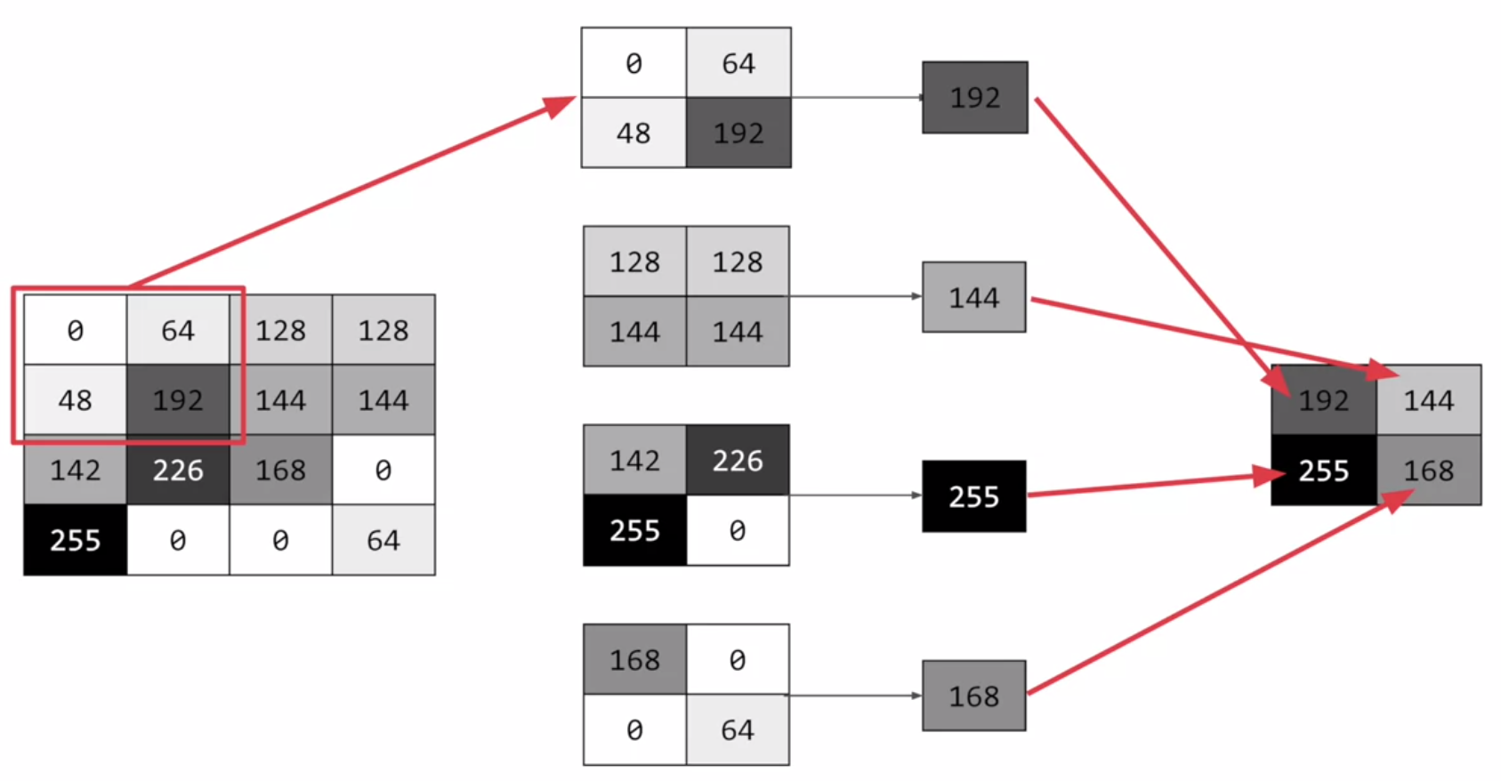
Well, if you've ever done any kind of image processing, it usually involves having a filter and passing that filter over the image in order to change the underlying image. The process works a little bit like this. For every pixel, take its value, and take a look at the value of its neighbors. If our filter is three by three, then we can take a look at the immediate neighbor, so that you have a corresponding three by three grid. Then to get the new value for the pixel, we simply multiply each neighbor by the corresponding value in the filter.
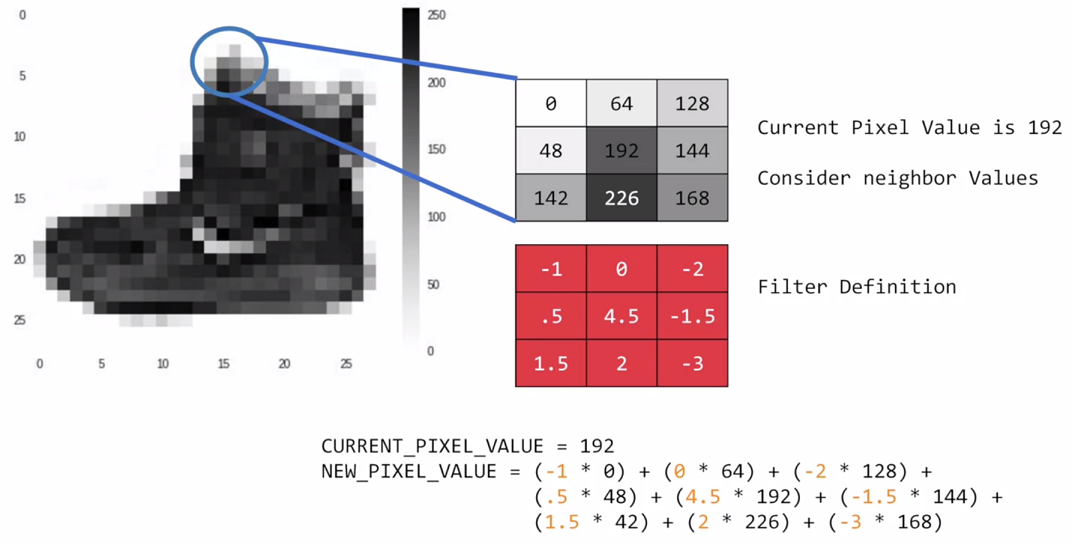
So, for example, in this case, our pixel has the value 192, and its upper left neighbor has the value zero. The upper left value and the filter is negative one, so we multiply zero by negative one. Then we would do the same for the upper neighbor. Its value is 64 and the corresponding filter value was zero, so we'd multiply those out. Repeat this for each neighbor and each corresponding filter value, and would then have the new pixel with the sum of each of the neighbor values multiplied by the corresponding filter value, and that's a convolution. It's really as simple as that.
The idea here is that some convolutions will change the image in such a way that certain features in the image get emphasized. So, for example, if you look at this filter, then the vertical lines in the image really pop out.
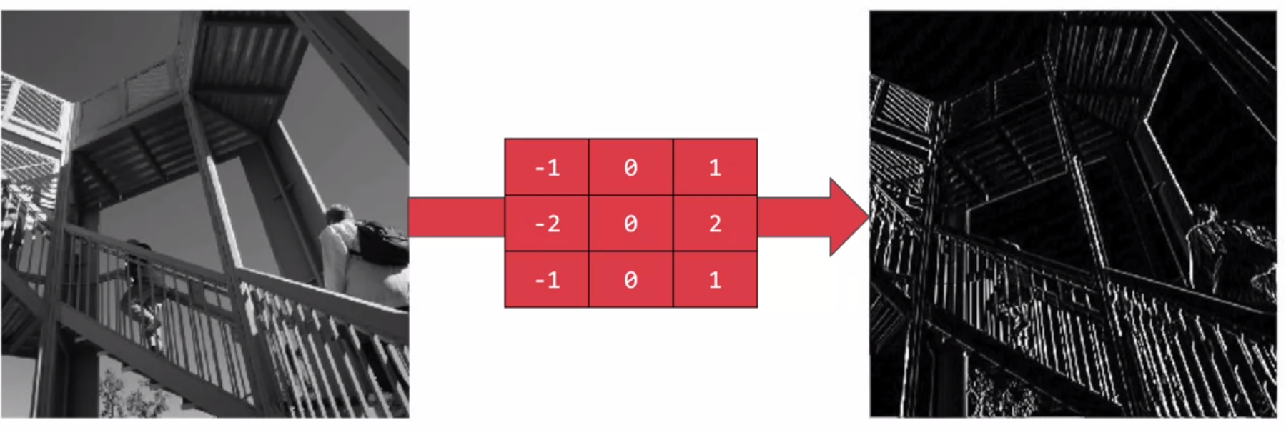
With this filter, the horizontal lines pop out.
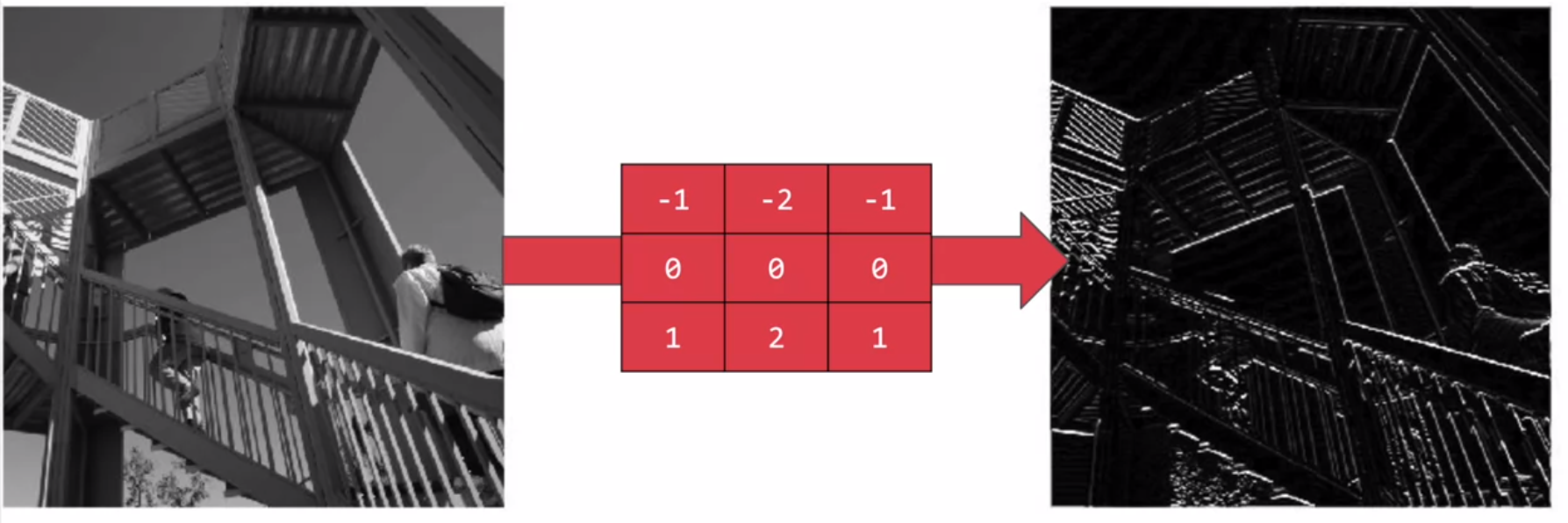
Now, that's a very basic introduction to what convolutions do, and when combined with something called pooling, they can become really powerful.
But simply, pooling is a way of compressing an image. A quick and easy way to do this, is to go over the image of four pixels at a time, i.e, the current pixel and its neighbors underneath and to the right of it. Of these four, pick the biggest value and keep just that. So, for example, you can see it here. My 16 pixels on the left are turned into the four pixels on the right, by looking at them in two-by-two grids and picking the biggest value.
This will preserve the features that were highlighted by th./deve convolution, while simultaneously quartering the size of the image. We have the horizontal and vertical axes.
# Implementing convolutional layers
So now let's take a look at convolutions and pooling in code. We don't have to do all the math for filtering and compressing, we simply define convolutional and pooling layers to do the job for us. So here's our code from the earlier example, where we defined out a neural network to have an input layer in the shape of our data, and output layer in the shape of the number of categories we're trying to define, and a hidden layer in the middle. The Flatten takes our square 28 by 28 images and turns them into a one dimensional array.
model = keras.Sequential([
    keras.layers.Flatten(),
    keras.layers.Dense(128, activation=tf.nn.relu),
    keras.layers.Dense(10, activation=tf.nn.softmax)
])
2
3
4
5
To add convolutions to this, you use code like this. You'll see that the last three lines are the same, the Flatten, the Dense hidden layer with 128 neurons, and the Dense output layer with 10 neurons. What's different is what has been added on top of this. Let's take a look at this, line by line.
model = keras.models.Sequential([
    keras.layers.Conv2D(64, (3, 3), activation=tf.nn.relu,
                        input_shape=(28, 28, 1)),
    keras.layers.MaxPooling2D(2, 2),
    keras.layers.Conv2D(64, (3, 3), activation=tf.nn.relu),
    keras.layers.MaxPooling2D(2, 2),
    keras.layers.Flatten(),
    keras.layers.Dense(128, activation=tf.nn.relu),
    keras.layers.Dense(128, activation=tf.nn.tanh),
    keras.layers.Dense(10, activation=tf.nn.softmax)
])
2
3
4
5
6
7
8
9
10
11
Here we're specifying the first convolution. We're asking keras to generate 64 filters for us. These filters are 3 by 3, their activation is relu, which means the negative values will be thrown way, and finally the input shape is as before, the 28 by 28. That extra 1 just means that we are tallying using a single byte for color depth. As we saw before our image is our gray scale, so we just use one byte.
    keras.layers.Conv2D(64, (3, 3), activation=tf.nn.relu,
                        input_shape=(28, 28, 1)),
2
Now, of course, you might wonder what the 64 filters are. It's a little beyond the scope of this class to define them, but they aren't random. They start with a set of known good filters in a similar way to the pattern fitting that you saw earlier, and the ones that work from that set are learned over time.
More details on CNN's
Convolutional Neural Networks (Course 4 of the Deep Learning Specialization)
# Implementing pooling layers
This next line of code will then create a pooling layer. It's max-pooling because we're going to take the maximum value. We're saying it's a two-by-two pool, so for every four pixels, the biggest one will survive as shown earlier.
keras.layers.MaxPooling2D(2, 2),
We then add another convolutional layer, and another max-pooling layer so that the network can learn another set of convolutions on top of the existing one, and then again, pool to reduce the size.
    keras.layers.Conv2D(64, (3, 3), activation=tf.nn.relu),
    keras.layers.MaxPooling2D(2, 2),
2
So, by the time the image gets to the flatten to go into the dense layers, it's already much smaller. It's being quartered, and then quartered again. So, its content has been greatly simplified, the goal being that the convolutions will filter it to the features that determine the output.
A really useful method on the model is the model.summary() method. This allows you to inspect the layers of the model, and see the journey of the image through the convolutions, and here is the output.
... model.summary()
...
Model: "sequential_5"
_________________________________________________________________
Layer (type)                 Output Shape              Param #
=================================================================
conv2d (Conv2D)              (None, 26, 26, 64)        640
_________________________________________________________________
max_pooling2d (MaxPooling2D) (None, 13, 13, 64)        0
_________________________________________________________________
conv2d_1 (Conv2D)            (None, 11, 11, 64)        36928
_________________________________________________________________
max_pooling2d_1 (MaxPooling2 (None, 5, 5, 64)          0
_________________________________________________________________
flatten_5 (Flatten)          (None, 1600)              0
_________________________________________________________________
dense_15 (Dense)             (None, 128)               204928
_________________________________________________________________
dense_16 (Dense)             (None, 128)               16512
_________________________________________________________________
dense_17 (Dense)             (None, 10)                1290
=================================================================
Total params: 260,298
Trainable params: 260,298
Non-trainable params: 0
_________________________________________________________________
2
3
4
5
6
7
8
9
10
11
12
13
14
15
16
17
18
19
20
21
22
23
24
25
26
It's a nice table showing us the layers, and some details about them including the output shape. It's important to keep an eye on the output shape column. When you first look at this, it can be a little bit confusing and feel like a bug. After all, isn't the data 28 by 28, so why is the output, 26 by 26?
The key to this is remembering that the filter is a three by three filter.
Consider what happens when you start scanning through an image starting on the top left.
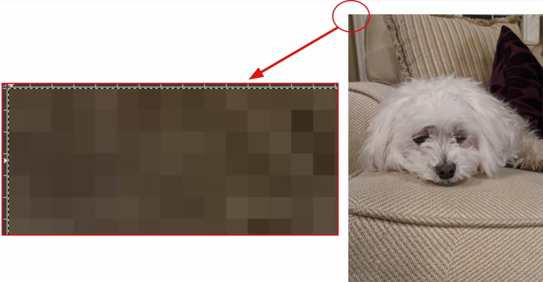
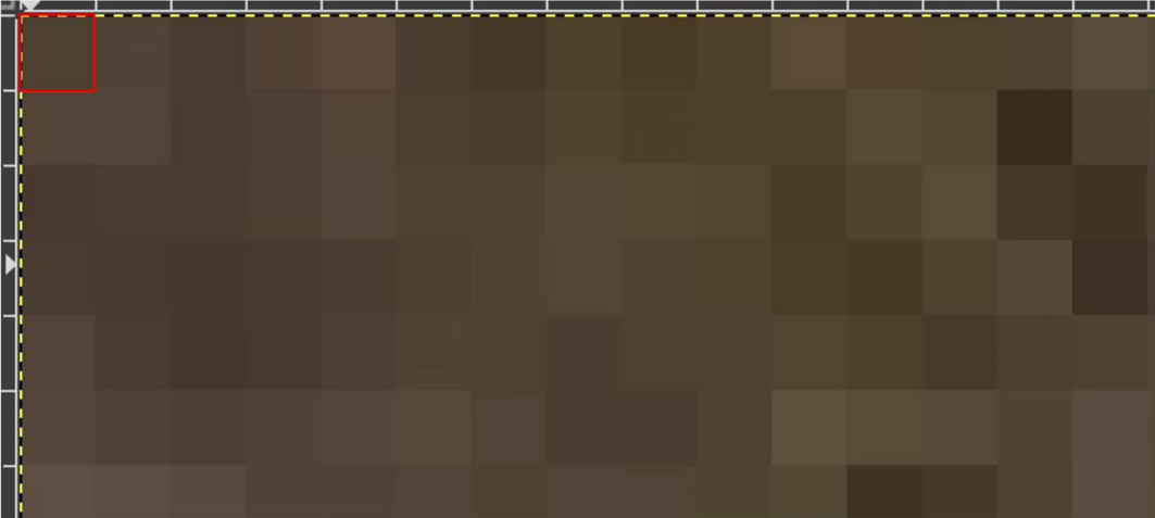
So, for example with this image of the dog on the right, you can see zoomed into the pixels at its top left corner.
You can't calculate the filter for the pixel in the top left, because it doesn't have any neighbors above it or to its left.
In a similar fashion, the next pixel to the right won't work either because it doesn't have any neighbors above it.
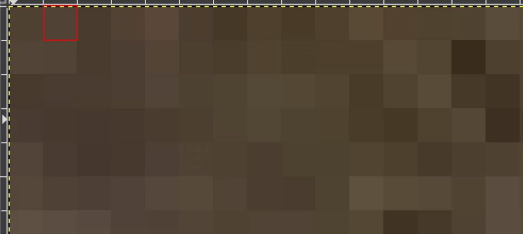
So, logically, the first pixel that you can do calculations on is this one, because this one of course has all eight neighbors that a three by three filter needs.
This when you think about it, means that you can't use a one pixel margin all around the image, so the output of the convolution will be two pixels smaller on x, and two pixels smaller on y.
If your filter is five-by-five for similar reasons, your output will be four smaller on x, and four smaller on y.
So, that's y with a three by three filter, our output from the 28 by 28 image, is now 26 by 26, we've removed that one pixel on x and y, and each of the borders.
So, next is the first of the max-pooling layers. Now, remember we specified it to be two-by-two, thus turning four pixels into one, and having our x and y. So, now our output gets reduced from 26 by 26, to 13 by 13.
_________________________________________________________________
Layer (type)                 Output Shape              Param #
=================================================================
conv2d (Conv2D)              (None, 26, 26, 64)        640
_________________________________________________________________
max_pooling2d (MaxPooling2D) (None, 13, 13, 64)        0
_________________________________________________________________
conv2d_1 (Conv2D)            (None, 11, 11, 64)        36928
_________________________________________________________________
max_pooling2d_1 (MaxPooling2 (None, 5, 5, 64)          0
_________________________________________________________________
flatten_5 (Flatten)          (None, 1600)              0
_________________________________________________________________
dense_15 (Dense)             (None, 128)               204928
_________________________________________________________________
dense_16 (Dense)             (None, 128)               16512
_________________________________________________________________
dense_17 (Dense)             (None, 10)                1290
=================================================================
Total params: 260,298
Trainable params: 260,298
Non-trainable params: 0
_________________________________________________________________
2
3
4
5
6
7
8
9
10
11
12
13
14
15
16
17
18
19
20
21
22
23
The convolutions will then operate on that, and of course, we lose the one pixel margin as before, so we're down to 11 by 11, add another two-by-two max-pooling to have this rounding down, and went down, down to five-by-five images. So, now our dense neural network is the same as before, but it's being fed with five-by-five images instead of 28 by 28 ones.
conv2d_1 (Conv2D)            (None, 11, 11, 64)        36928
_________________________________________________________________
max_pooling2d_1 (MaxPooling2 (None, 5, 5, 64)          0
2
3
But remember, it's not just one compress five-by-five image instead of the original 28 by 28, there are a number of convolutions per image that we specified, in this case 64. So, there are 64 new images of five-by-five that had been fed in. Flatten that out and you have 25 pixels times 64, which is 1600.
So, you can see that the new flattened layer has 1,600 elements in it, as opposed to the 784 that you had previously. This number is impacted by the parameters that you set when defining the convolutional 2D layers.
flatten_5 (Flatten) (None, 1600) 0
Later when you experiment, you'll see what the impact of setting what other values for the number of convolutions will be, and in particular, you can see what happens when you're feeding less than 784 over all pixels in. Training should be faster, but is there a sweet spot where it's more accurate? Well, let's switch to the workbook, and we can try it out for ourselves.
# Improving the Fashion classifier with convolutions
In the previous video, you looked at convolutions and got a glimpse for how they worked. By passing filters over an image to reduce the amount of information, they then allowed the neural network to effectively extract features that can distinguish one class of image from another. You also saw how pooling compresses the information to make it more manageable. This is a really nice way to improve our image recognition performance.
import tensorflow as tf
print(tf.__version__)
from tensorflow import keras

import time
from tensorflow.keras.callbacks import TensorBoard

NAME = "FashionMNIST-CNN".format(int(time.time()))
tensorboard = TensorBoard(log_dir='logs/{}'.format(NAME))

mnist = keras.datasets.fashion_mnist

(training_images, training_labels), (test_images, test_labels) = mnist.load_data()

training_images = training_images.reshape(60000, 28, 28, 1)
training_images = training_images / 255.0

test_images = test_images.reshape(10000, 28, 28, 1)
test_images = test_images / 255.0


model = keras.models.Sequential([
    keras.layers.Conv2D(64, (3, 3), activation=tf.nn.relu,
                        input_shape=(28, 28, 1)),
    keras.layers.MaxPooling2D(2, 2),
    keras.layers.Conv2D(64, (3, 3), activation=tf.nn.relu),
    keras.layers.MaxPooling2D(2, 2),
    keras.layers.Flatten(),
    keras.layers.Dense(128, activation=tf.nn.relu),
    keras.layers.Dense(10, activation=tf.nn.softmax)
])


model.summary()
model.compile(optimizer='adam',
              loss='sparse_categorical_crossentropy')

model.fit(training_images, training_labels, epochs=5)
2
3
4
5
6
7
8
9
10
11
12
13
14
15
16
17
18
19
20
21
22
23
24
25
26
27
28
29
30
31
32
33
34
35
36
37
38
Here's the same neural network that you used before for loading the set of images of clothing and then classifying them. By the end of epoch five, you can see the loss is around 0.29, meaning, your accuracy is pretty good on the training data. It took just a few seconds to train, so that's not bad. With the test data as before and as expected, the losses a little higher and thus, the accuracy is a little lower. So now, you can see the code that adds convolutions and pooling. We're going to do two convolutional layers each with 64 convolution, and each followed by a max pooling layer. You can see that we defined our convolutions to be three-by-three and our pools to be two-by-two. Let's train. The first thing you'll notice is that the training is much slower. For every image, 64 convolutions are being tried, and then the image is compressed and then another 64 convolutions, and then it's compressed again, and then it's passed through the DNN, and that's for 60,000 images that this is happening on each epoch. So it might take a few minutes instead of a few seconds.
Model: "sequential_8"
_________________________________________________________________
Layer (type)                 Output Shape              Param #
=================================================================
conv2d_6 (Conv2D)            (None, 26, 26, 64)        640
_________________________________________________________________
max_pooling2d_6 (MaxPooling2 (None, 13, 13, 64)        0
_________________________________________________________________
conv2d_7 (Conv2D)            (None, 11, 11, 64)        36928
_________________________________________________________________
max_pooling2d_7 (MaxPooling2 (None, 5, 5, 64)          0
_________________________________________________________________
flatten_8 (Flatten)          (None, 1600)              0
_________________________________________________________________
dense_24 (Dense)             (None, 128)               204928
_________________________________________________________________
dense_25 (Dense)             (None, 10)                1290
=================================================================
Total params: 243,786
Trainable params: 243,786
Non-trainable params: 0
_________________________________________________________________
Epoch 1/5
1875/1875 [==============================] - 36s 19ms/step - loss: 0.4388
Epoch 2/5
1875/1875 [==============================] - 36s 19ms/step - loss: 0.2921
Epoch 3/5
1875/1875 [==============================] - 36s 19ms/step - loss: 0.2503
Epoch 4/5
1875/1875 [==============================] - 36s 19ms/step - loss: 0.2169
Epoch 5/5
1875/1875 [==============================] - 36s 19ms/step - loss: 0.1922
model.evaluate(test_images, test_labels)
313/313 [==============================] - 1s 5ms/step - loss: 0.2572
0.2572135925292969
2
3
4
5
6
7
8
9
10
11
12
13
14
15
16
17
18
19
20
21
22
23
24
25
26
27
28
29
30
31
32
33
34
35
36
TIP
The number of steps per epoch is equal to ceil(samples / batch_size). The default batch size in model.fit() is 32 (documentation). If the MNIST training data has 60000 samples, then each epoch would take 60000 / 32 = 1875 steps.
If we adjust the batch_size to 1 we get all of the 60000 steps.
model.fit(training_images, training_labels, epochs=5, batch_size=1)
As you can see it took much longer.
As you can see it's taken much longer.
Epoch 1/5
60000/60000 [==============================] - 107s 2ms/step - loss: 0.4083
Epoch 2/5
60000/60000 [==============================] - 121s 2ms/step - loss: 0.3205
Epoch 3/5
60000/60000 [==============================] - 132s 2ms/step - loss: 0.3052
Epoch 4/5
60000/60000 [==============================] - 117s 2ms/step - loss: 0.2996
Epoch 5/5
60000/60000 [==============================] - 114s 2ms/step - loss: 0.2949
model.evaluate(test_images, test_labels)
313/313 [==============================] - 2s 5ms/step - loss: 0.3771
0.3771289885044098
2
3
4
5
6
7
8
9
10
11
12
13
14
Now that it's done, you can see that the loss has improved a little. In this case, it's brought our accuracy up a bit for both our test data and with our training data. That's pretty cool, right?
Now, let's take a look at the code at the bottom of the notebook. Now, this is a really fun visualization of the journey of an image through the convolutions. First, I'll print out the first 100 test labels. The number nine as we saw earlier is a shoe or boots. I picked out a few instances of this whether the zero, the 23rd and the 28th labels are all nine. So let's take a look at their journey.
>>>print(test_labels[:100])

[9 2 1 1 6 1 4 6 5 7 4 5 7 3 4 1 2 4 8 0 2 5 7 9 1 4 6 0 9 3 8 8 3 3 8 0 7
 5 7 9 6 1 3 7 6 7 2 1 2 2 4 4 5 8 2 2 8 4 8 0 7 7 8 5 1 1 2 3 9 8 7 0 2 6
 2 3 1 2 8 4 1 8 5 9 5 0 3 2 0 6 5 3 6 7 1 8 0 1 4 2]
2
3
4
5
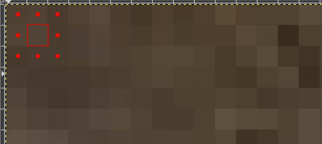
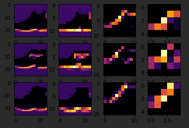
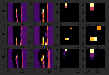
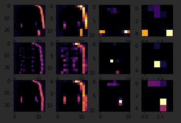
The Keras API gives us each convolution and each pooling and each dense, etc. as a layer. So with the layers API, I can take a look at each layer's outputs, so I'll create a list of each layer's output. I can then treat each item in the layer as an individual activation model if I want to see the results of just that layer. Now, by looping through the layers, I can display the journey of the image through the first convolution and then the first pooling and then the second convolution and then the second pooling. Note how the size of the image is changing by looking at the axes.
FIRST_IMAGE = 4
SECOND_IMAGE = 7
THIRD_IMAGE = 26
CONVOLUTION_NUMBER = 1
2
3
4
So, for example, if I change the third image to be one, which looks like a handbag, you'll see that it also has a bright line near the bottom that could look like the soul of the shoes, but by the time it gets through the convolutions, that's lost, and that area for the laces doesn't even show up at all. So this convolution definitely helps me separate issue from a handbag. Again
if I said it's a two, it appears to be trousers, but the feature that detected something that the shoes had in common fails again.
Also, if I changed my third image back to that for shoe, but I tried a different convolution number, you'll see that for convolution two, it didn't really find any common features.
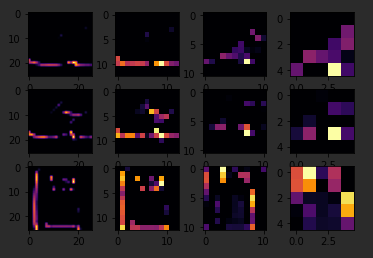
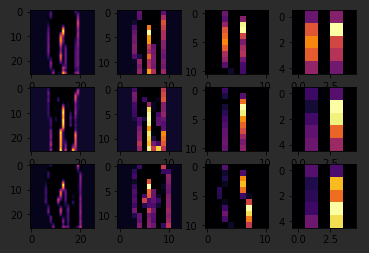
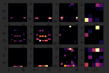
To see commonality in a different image, try images two, three, and five. These all appear to be trousers.
Convolutions two and four seem to detect this vertical feature as something they all have in common.
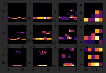
If I again go to the list and find three labels that are the same, in this case six, I can see what they signify. When I run it, I can see that they appear to be shirts.
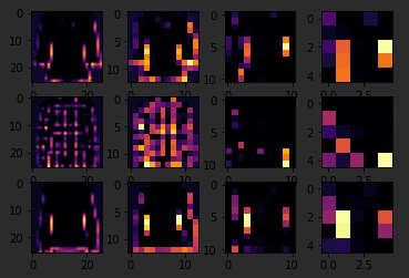
Convolution four doesn't do a whole lot, so let's try five. We can kind of see that the color appears to light up in this case.
Let's try convolution one.
I don't know about you, but I can play with this all day.
Then see what you do when you run it for yourself. When you're done playing, try tweaking the code with these suggestions, editing the convolutions, removing the final convolution, and adding more, etc. Also, in a previous exercise, you added a callback that finished training once the loss had a certain amount. So try to add that here. When you're done, we'll move to the next stage, and that's dealing with images that are larger and more complex than these ones. To see how convolutions can maybe detect features when they aren't always in the same place, like they would be in these tightly controlled 28 by 28 images.
# Walking through convolutions
In the previous lessons, you saw the impacts that convolutions and pooling had on your networks efficiency and learning, but a lot of that was theoretical in nature. So I thought it'd be interesting to hack some code together to show how a convolution actually works. We'll also create a little pooling algorithm, so you can visualize its impact. There's a notebook that you can play with too, and I'll step through that here.
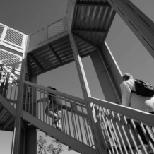
It does use a few Python libraries that you may not be familiar with such as cv2. It also has Matplotlib that we used before. If you haven't used them, they're really quite intuitive for this task and they're very very easy to learn. So first, we'll set up our inputs and in particular, import the misc library from SciPy. Now, this is a nice shortcut for us because misc.ascent returns a nice image that we can play with, and we don't have to worry about managing our own.
import cv2
import numpy as np
from scipy import misc
i = misc.ascent()
2
3
4
Matplotlib contains the code for drawing an image and it will render it right in the browser with Colab. Here, we can see the ascent image from SciPy.
import matplotlib.pyplot as plt
plt.grid(False)
plt.gray()
plt.axis('off')
plt.imshow(i)
plt.show()
2
3
4
5
6
Next up, we'll take a copy of the image, and we'll add it with our homemade convolutions, and we'll create variables to keep track of the x and y dimensions of the image.
i_transformed = np.copy(i)
size_x = i_transformed.shape[0]
size_y = i_transformed.shape[1]
2
3
So we can see here that it's a 512 by 512 image. So now, let's create a convolution as a three by three array. We'll load it with values that are pretty good for detecting sharp edges first.
filter = [[0, 1, 1], [1, -4, 1], [0, 1, 0]]
Here's where we'll create the convolution. We iterate over the image, leaving a one pixel margin. You'll see that the loop starts at one and not zero, and it ends at size x minus one and size y minus one. In the loop, it will then calculate the convolution value by looking at the pixel and its neighbors, and then by multiplying them out by the values determined by the filter, before finally summing it all up.
for x in range(1, size_x-1):
    for y in range(1, size_y-1):
        convolution = 0.0
        convolution = convolution + (i[x - 1, y - 1] * filter[0][0])
        convolution = convolution + (i[x,     y - 1] * filter[0][1])
        convolution = convolution + (i[x + 1, y - 1] * filter[0][2])
        convolution = convolution + (i[x - 1, y    ] * filter[1][1])
        convolution = convolution + (i[x    , y    ] * filter[1][2])
        convolution = convolution + (i[x + 1, y    ] * filter[1][0])
        convolution = convolution + (i[x - 1, y + 1] * filter[2][0])
        convolution = convolution + (i[x    , y + 1] * filter[2][1])
        convolution = convolution + (i[x + 1, y + 1] * filter[2][2])
        if convolution<0:
            convolution=0
        if convolution<255:
            convolution=255
        i_transformed[x, y] = convolution
2
3
4
5
6
7
8
9
10
11
12
13
14
15
16
17
Let's run it. It takes just a few seconds, so when it's done, let's draw the results. We can see that only certain features made it through the filter. I've provided a couple more filters, so let's try them.
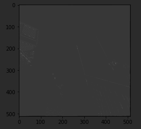
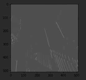
This first one is really great at spotting vertical lines. So when I run it, and plot the results, we can see that the vertical lines in the image made it through. It's really cool because they're not just straight up and down, they are vertical in perspective within the perspective of the image itself.
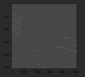
Similarly, this filter works well for horizontal lines. So when I run it, and then plot the results, we can see that a lot of the horizontal lines made it through.
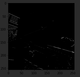
Now, let's take a look at pooling, and in this case, Max pooling, which takes pixels in chunks of four and only passes through the biggest value. I run the code and then render the output. We can see that the features of the image are maintained, but look closely at the axes, and we can see that the size has been halved from the 500's to the 250's.
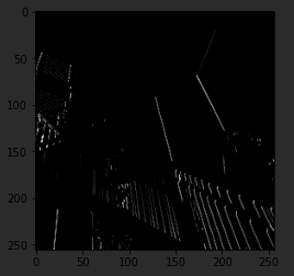
For fun, we can try the other filter, run it, and then compare the convolution with its pooled version. Again, we can see that the features have not just been maintained, they may have also been emphasized a bit.
So that's how convolutions work. Under the hood, TensorFlow is trying different filters on your image and learning which ones work when looking at the training data.
As a result, when it works, you'll have greatly reduced information passing through the network, but because it isolates and identifies features, you can also get increased accuracy.
Have a play with the filters in this workbook and see if you can come up with some interesting effects of your own.