Tensorflow

Simple Linear Regression.

Minimal Example

1. Import the relevant libraries

import numpy as np
import matplotlib.pyplot as plt
from mpl_toolkits.mplot3d import Axes3D

2. Generate random input data to train on

observations = 1000
xs = np.random.uniform(low=-10, high=10, size=(observations, 1))
zs = np.random.uniform(-10,10,(observations, 1))

inputs = np.column_stack((xs, zs))

print(inputs.shape)
print(inputs)

Output is a matrix of size (1000,2)

(1000, 2)

[[ 7.44651066  3.0441044 ]
 [ 3.18741031 -6.10663328]
 [ 7.47234553  6.86829353]
 ...
 [ 4.3408767   2.59859389]
 [ 5.96692549 -1.95235124]
 [ 6.43664934 -8.52279315]]

Elements of the model in supervised learning	Status
inputs	done
weights	Computer
biases	Computer
outputs	Computer
targets	to do

Targets = $f(x,z) = 2x - 3z + 5 + noise$

Where 2 is the first weight$(W_1)$ 3 is the second weight$(W_2)$ and 5$(b)$ is the baias.

The noise is introduced to randomize the data.

3. Create the targets we will aim at

noise = np.random.uniform(-1, 1, (observations, 1))

targets = 2*xs - 3*zs + 5 + noise

# the targets are a linear combination of two vectors 1000x1 
# a scalar and noise 1000x1, their shape should be 1000x1

print(targets.shape)

Output the shape of the targets, a matrix 1000x1

(1000, 1)

4. Plot the training data

# In order to use the 3D plot, the objects should have a certain shape, so we reshape the targets.
# The proper method to use is reshape and takes as arguments the dimensions in which we want to fit the object.
targets = targets.reshape(observations,)

# Plotting according to the conventional matplotlib.pyplot syntax

# Declare the figure
fig = plt.figure()

# A method allowing us to create the 3D plot
ax = fig.add_subplot(111, projection='3d')

# Choose the axes.
ax.plot(xs, zs, targets)

# Set labels
ax.set_xlabel('xs')
ax.set_ylabel('zs')
ax.set_zlabel('Targets')

# You can fiddle with the azim parameter to plot the data from different angles. Just change the value of azim=100
# to azim = 0 ; azim = 200, or whatever. Check and see what happens.
ax.view_init(azim=100)

# So far we were just describing the plot. This method actually shows the plot. 
plt.show()

# We reshape the targets back to the shape that they were in before plotting.
# This reshaping is a side-effect of the 3D plot. Sorry for that.
targets = targets.reshape(observations,1)

Clean code

targets = targets.reshape(observations,)
fig = plt.figure()
ax = fig.add_subplot(111, projection='3d')
ax.plot(xs, zs, targets)
ax.set_xlabel('xs')
ax.set_ylabel('zs')
ax.set_zlabel('Targets')
ax.view_init(azim=100)
plt.show()
targets = targets.reshape(observations, 1)

5. Create weights

# our initial weights and biases will be picked randomly from
# the interval minus 0.1 to 0.1.
init_range = 0.1
#The size of the weights matrix is two by one as we
# have two variables so there are two weights one for#
#each input variable and a single output.
weights = np.random.uniform(-init_range, init_range, size=(2, 1))

print(f'Weights: {weights}')

6. Create Biases

#Let's declare the bias and illogically the appropriate shape is one by one.
#So the bias is a scalar in machine learning.
#There are many biases as there are outputs.
#Each bias refers to an output.
biases = np.random.uniform(-init_range, init_range, size=1)

print(f'Biases: {biases}')

Weights: [[-0.07021836]
 [ 0.00626743]]
Biases: [-0.01464248]

7. Set a learning rate

learning_rate = 0.02

So we are all set. We have inputs targets and arbitrary numbers for weights and biases. What is left is to vary the weights and biases so our outputs are closest to the targets as we know by now. The problem boils down to minimizing the loss function with respect to the weights and the biases. And because this is a regression we'll use one half the L2 norm loss function.

Next let's make our model learn.

Since this is an iterative problem. We must create a loop which will apply our update rule and calculate the last function.

I'll use a for loop with 100 iterations to complete this task. Let's see the game plan will follow:

• At each iteration We will calculate the outputs

• and compare them to the targets through the last function.

• We will print the last for each iteration so we know how the algorithm is doing.

• Finally we will adjust the weights and biases to get a better fit of the data.

• At the next iteration these updated weights and biases will provide different outputs.

• Then the procedure will be repeated.

Now the dot product of the input times the weights is 1000 by two times to buy one. So a 1000 by 1 matrix when we add the bias which is a scalar. Python adds the element wise. This means it is added to each element of the output matrix.

for i in range(100):
    outputs = np.dot(inputs, weights) + biases

OK for simplicity let's declare a variable called deltas which will record the difference between the outputs and the targets. We already introduce such variable in the gradient descent lecture deltas equals outputs minus targets. That's useful as it is a part of the update rule. Then we must calculate the loss.

deltas = outputs - targets

L2-norm loss formula:

$\sum _i(y_i - t_i)^2$

We said we will use half the L2 norm loss. Python actually speaking deltas is a 1000 by one array. We are interested in the sum of its terms squared. Following the formula for the L2 norm loss there is a num PI method called sum which will allow us to sum all the values in the array the L2 norm requires these values to be squared. So the code looks like this. And P does some of Delta squared. We then divide the whole expression by two to get the elegant update rules from the gradient descent. Let's further augment the loss by dividing it by the number of observations we have. This would give us the average loss per observation or the mean loss. Similarily to the division by 2. This does not change the logic of the last function. It is still lower than some more accurate results that will be obtained. This little improvement makes the learning independent of the number of observations instead of adjusting the learning rate. We adjust the loss that that's valuable as the same learning rate should give us similar results for both 1000 and 1 million observations.

loss = np.sum(deltas ** 2) / 2 / observations

We'll print the last we've obtained each step. That's done as we want to keep an eye on whether it is decreasing as iterations are performed. If it is decreasing our machine learning algorithm functions well.

print(loss)

Finally we must update the weights and biases so they are ready for the next iteration using the same rescaling trick. I'll also reskill the deltas. This is yet another way to make the algorithm more universal. So the new variable is deltas underscored skilled and equals deltas divided by observations.

deltas_scaled = deltas / observations

Let's update the weights. We will follow the gradient descent logic.

$w_{i+1} = w_i - \eta \sum _i x_i \delta_i$

The new weights are equal to the old weights minus the learning rate times the dot product of the inputs and the Deltas underscored scaled. The shape of the weights is two by one the shape of the inputs is one thousand by two and that of the Delta skilled is one thousand by one. Obviously we cannot simply multiply the inputs and the deltas. This is an issue that may arise occasionally due to the linear algebra involved to fix it. We must transpose the inputs matrix using the object but the method. Now the major C's are compatible. By 1000 times 1000 by one is equal to 2 by 1.

weights = weights - learning_rate * np.dot(inputs.T, deltas_scaled)

TIP

Often when dealing with matrices you find the correct way to code it through dimensionality checks and compatability errors.

However transposing major C's doesn't affect the information they hold so we can do it freely.

All right let's update the biases. The new biases are equal to the old biases minus the learning rate times the sum of the deltas as explained in the gradient descent lecture.

biases = biases - learning_rate * np.sum(deltas_scaled)

This is the entire algorithm. Let's recap what it does:

1. first it calculates the outputs forgiven weights and biases.
2. Second it calculates a loss function that compares the outputs to the targets.
3. Third it prints the loss. So we can later analyze it and
4. forth, We update the weights and the bias is following the gradient descent methodology.

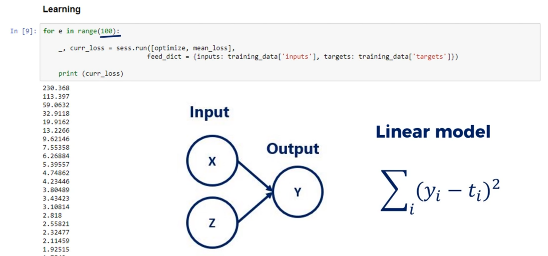
Let's run the code. What we get is a list of numbers that appears to be in descending order right. These are the values of our average last function. It started from a high value and at each iteration it became lower and lower until it reached a point where it almost stopped changing. This means we have minimized or almost minimize the loss function with respect to the weights and biases. Therefore we have found a linear function that fits the model Well

113.1346113499832
108.21425084240616
103.88888353315217
99.7849517016046
95.84949440054764
92.0702726846745
88.4404105995388
84.95392016265656
81.60512775430881
78.38859366840362
75.29909427907384
72.33161242080419
69.4813290972211
66.74361563721006
64.11402617596718
61.58829043492039
59.162306787044116
56.83213559608488
54.59399281885322
52.444243860188884
50.3793976706198
48.39610107712963
46.491133337827655
44.66140091167794
42.90393243479416
41.21587389514219
39.594483997814095
38.03712971334737
36.54128200186008
35.104511706058084
33.72448560644502
32.39896263232881
31.125790222471856
29.902900829474543
28.728308562215652
27.600105960897142
26.516460899456188
25.475613610314117
24.475873826630895
23.515618037423987
22.593286851094458
21.707382463078588
20.856466223512808
20.03915630096189
19.25412543841651
18.500098797916074
17.77585189029656
17.080208586701485
16.41203920862674
15.77025869339785
15.153824832100188
14.561736577101016
13.993032416414623
13.446788812270727
12.922118701350518
12.418170054254773
11.934124491864695
11.469195956348635
11.022629434656377
10.59369973242813
10.181710296327049
9.785992082882911
9.40590247200998
9.040824223434672
8.690164474338356
8.353353776587563
8.029845171988013
7.719113304060869
7.42065356489872
7.133981275715881
6.858630899762206
6.594155286322381
6.34012494457287
6.096127346117317
5.861766255067884
5.636661084584468
5.420446278826976
5.212770719316917
5.013297154744328
4.8217016532940695
4.637673076602049
4.460912574487216
4.291133099638719
4.128058941470141
3.9714252783838333
3.8209777477182216
3.676472032679767
3.537673465588702
3.4043566467943345
3.276305078640973
3.153310813890127
3.0351741180280087
2.921703144909945
2.812713625215003
2.7080285672048383
2.607477969300881
2.5108985440130636
2.4181334527717953
2.3290320512325318
2.2434496446393806

The weights and the biases are optimize. But so are the outputs. Since the optimization process has ended. We can check these values here. We observe the values from the last iteration of the for loop. The one that gave us the lowest last function in the memory of the computer the weights biases and outputs variables are optimized as of now. Congratulations you learn how to create your first machine learning algorithm.

Still let's spend an extra minute on that. I'd like to print the weights and the bias's the weights seem about right. The bias is close to five as we wanted but not really. That's because we use too few iterations or an inappropriate learning rate. Let's rerun the code for the loop. This will continue optimizing the algorithm for another hundred iterations. We can see the bias improves when we increase the number of iterations. We strongly encourage you to play around with the code and find the optimal number of iterations for the problem. Try different values for observations learning rate number of iterations maybe even initial range for initializing the weights and biases cool.

print(f'Weights: {weights}')
print(f'Biases: {biases}')

Targets = $f(x,z) = 2x - 3z + 5 + noise$

Weights: [[ 1.9962384 ]
 [-3.00212515]]
Biases: [5.28171043]

Weights: [[ 1.99842328]
 [-3.00330109]]
Biases: [5.01471378]

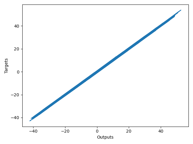
Finally I'd like to show you the plot of the output at the last iteration against the targets. The closer this plot is to a 45 degree line the closer the outputs are to the targets. Obviously our model worked like a charm.

Solving the simple example using TensorFlow

#%%
import numpy as np
import matplotlib.pyplot as plt
import tensorflow as tf

#%%
# 2. Data generation

observations = 1000
xs = np.random.uniform(low=-10, high=10, size=(observations, 1))
zs = np.random.uniform(-10, 10, (observations, 1))

generated_inputs = np.column_stack((xs, zs))

noise = np.random.uniform(-1, 1, (observations, 1))

generated_targets = 2*xs - 3*zs + 5 + noise

np.savez('TF_intro', inputs=generated_inputs, targets=generated_targets)
#%%
# 3. Solving with TensorFlow

training_data = np.load('TF_intro.npz')

input_size = 2
output_size = 1

# tf.keras.Sequential() function that specifies how the model
# will be laid down ('stack layers')
# Linear combination + Output = Layer*

# The tf.keras.layers.Dense(output size)
# takes the inputs provided to the model
# and calculates the dot product of the inputs and weights and adds the bias
# It would be the output = np.dot(inputs, weights) + bias

model = tf.keras.Sequential([
    tf.keras.layers.Dense(output_size)
])

# model.compile(optimizer, loss) configures the model for training
# https://www.tensorflow.org/api_docs/python/tf/keras/optimizers
# L2-norm loss = Least sum of squares (least sum of squared error)
# scaling by #observations = average (mean)

model.compile(optimizer='sgd', loss='mean_squared_error')

# What we've got left is to indicate to the model which data to fit
# modelf.fit(inouts, targets) fits (trains) the model.
# Epoch = iteration over the full dataset

model.fit(training_data['inputs'], training_data['targets'], epochs=100, verbose=2)


#%%
# 4. Extract the weights and bias

model.layers[0].get_weights()

weights = model.layers[0].get_weights()[0]
print(f'weights: {weights}')

biases = model.layers[0].get_weights()[1]
print(f'biases: {biases}')

#%%

# 5. Extract the outputs (make predictions)
# model.predict_on_batch(data) calculates the outputs given inputs
# these are the values that were compared to the targets to evaluate the loss function
print(model.predict_on_batch(training_data['inputs']).round(1))

print(training_data['targets'].round(1))

#%%

# 6. Plotting
# The line should be as close to 45 as possible
plt.plot(np.squeeze(model.predict_on_batch(training_data['inputs'])), np.squeeze(training_data['targets']))
plt.xlabel('Outputs')
plt.ylabel('Targets')
plt.show()

Making the model closer to the Numpy example

import numpy as np
import matplotlib.pyplot as plt
import tensorflow as tf

#%%
# 2. Data generation

observations = 1000
xs = np.random.uniform(low=-10, high=10, size=(observations, 1))
zs = np.random.uniform(-10, 10, (observations, 1))

generated_inputs = np.column_stack((xs, zs))

noise = np.random.uniform(-1, 1, (observations, 1))

generated_targets = 2*xs - 3*zs + 5 + noise

np.savez('TF_intro', inputs=generated_inputs, targets=generated_targets)
#%%
# 3. Solving with TensorFlow

training_data = np.load('TF_intro.npz')

input_size = 2
output_size = 1

# tf.keras.Sequential() function that specifies how the model
# will be laid down ('stack layers')
# Linear combination + Output = Layer*

# The tf.keras.layers.Dense(output size)
# takes the inputs provided to the model
# and calculates the dot product of the inputs and weights and adds the bias
# It would be the output = np.dot(inputs, weights) + bias

# tf.keras.layers.Dense(output_size, kernel_initializer, bias_initializer)
# function that is laying down the model (used tp 'stack layers') and initialize weights

model = tf.keras.Sequential([
    tf.keras.layers.Dense(output_size,
                          kernel_initializer=tf.random_uniform_initializer(minval=-0.1, maxval=0.1),
                          bias_initializer=tf.random_uniform_initializer(minval=-0.1, maxval=0.1))
])

custom_optimizer = tf.keras.optimizers.SGD(learning_rate=0.02)

# model.compile(optimizer, loss) configures the model for training
# https://www.tensorflow.org/api_docs/python/tf/keras/optimizers
# L2-norm loss = Least sum of squares (least sum of squared error)
# scaling by #observations = average (mean)

model.compile(optimizer=custom_optimizer, loss='mean_squared_error')

# What we've got left is to indicate to the model which data to fit
# modelf.fit(inouts, targets) fits (trains) the model.
# Epoch = iteration over the full dataset

model.fit(training_data['inputs'], training_data['targets'], epochs=100, verbose=2)


#%%
# 4. Extract the weights and bias

model.layers[0].get_weights()

weights = model.layers[0].get_weights()[0]
print(f'weights: {weights}')

biases = model.layers[0].get_weights()[1]
print(f'biases: {biases}')

#%%

# 5. Extract the outputs (make predictions)
# model.predict_on_batch(data) calculates the outputs given inputs
# these are the values that were compared to the targets to evaluate the loss function
print(model.predict_on_batch(training_data['inputs']).round(1))

print(training_data['targets'].round(1))

#%%

# 6. Plotting
# The line should be as close to 45 as possible
plt.plot(np.squeeze(model.predict_on_batch(training_data['inputs'])), np.squeeze(training_data['targets']))
plt.xlabel('Outputs')
plt.ylabel('Targets')
plt.show()

Going deeper Introduction to deep neural networks

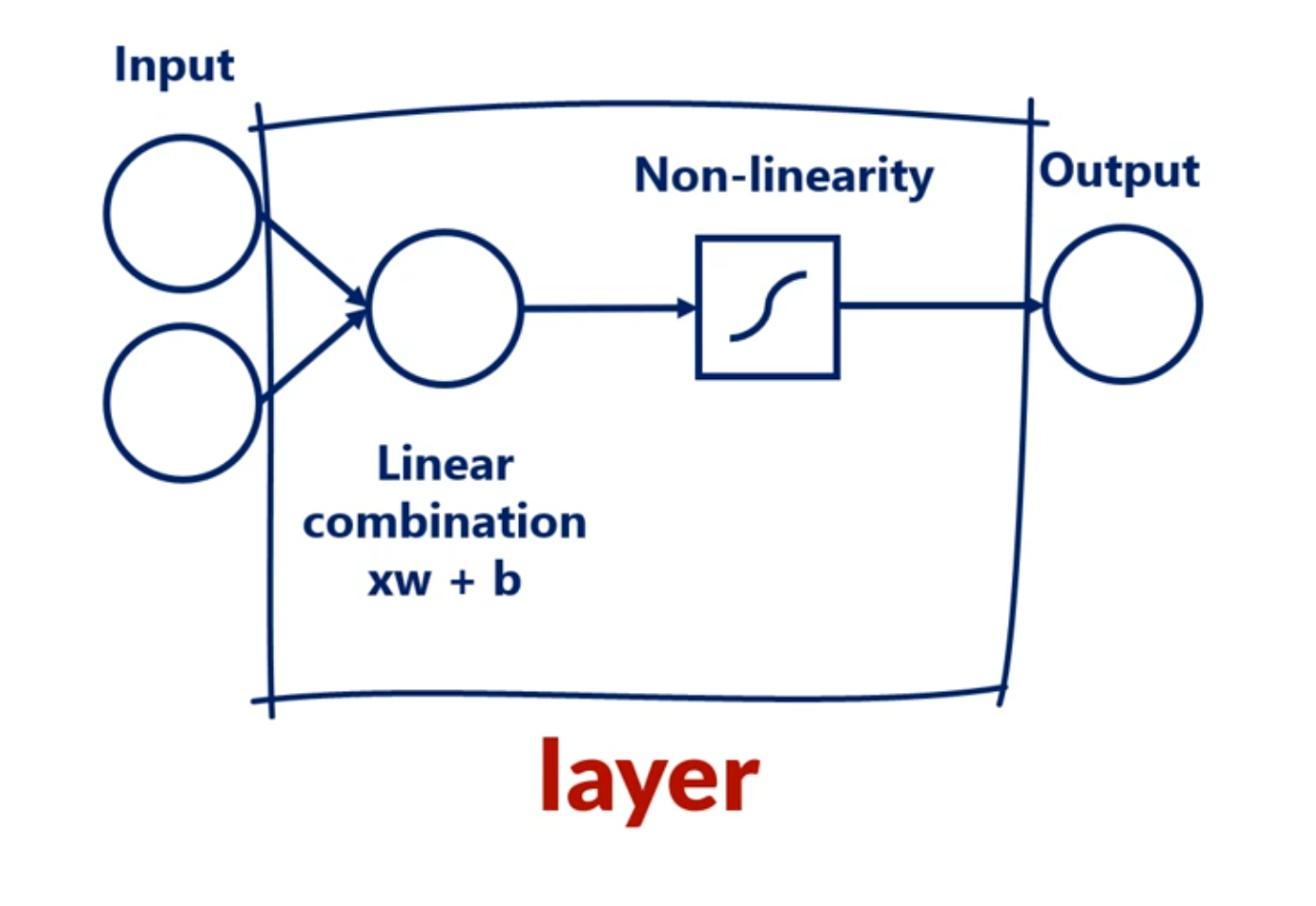
Layers

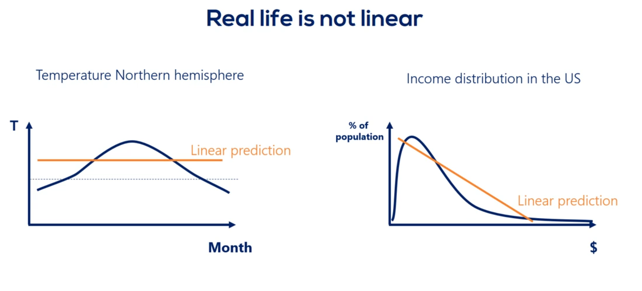
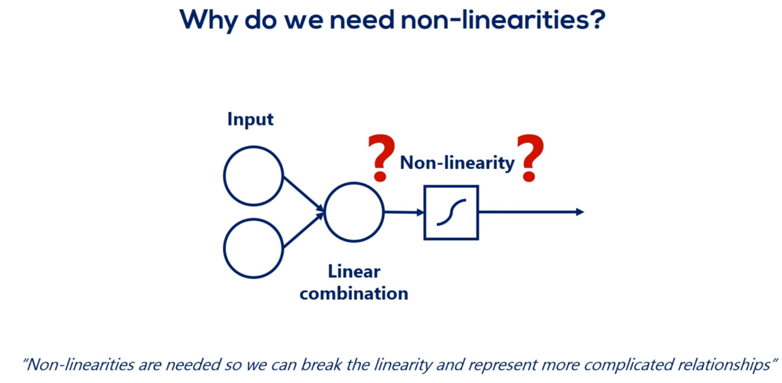
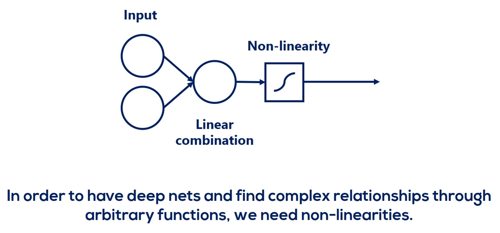
Mixing linear combinations and non-linearities allows us to model arbitrary functions.

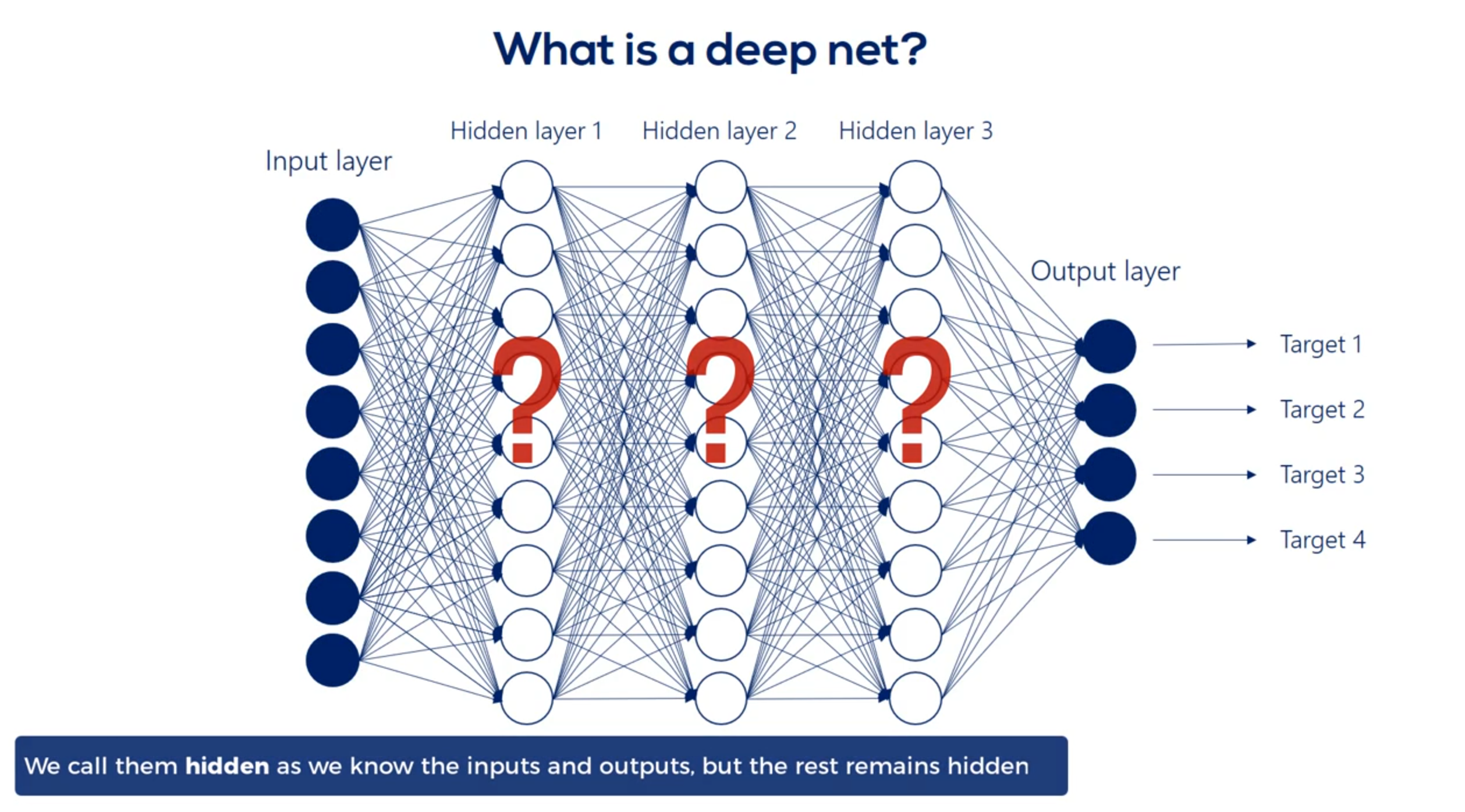
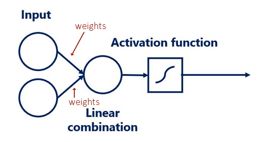
The layer is the building block of neural networks. The initial linear combinations and the added non-linearity form a layer.

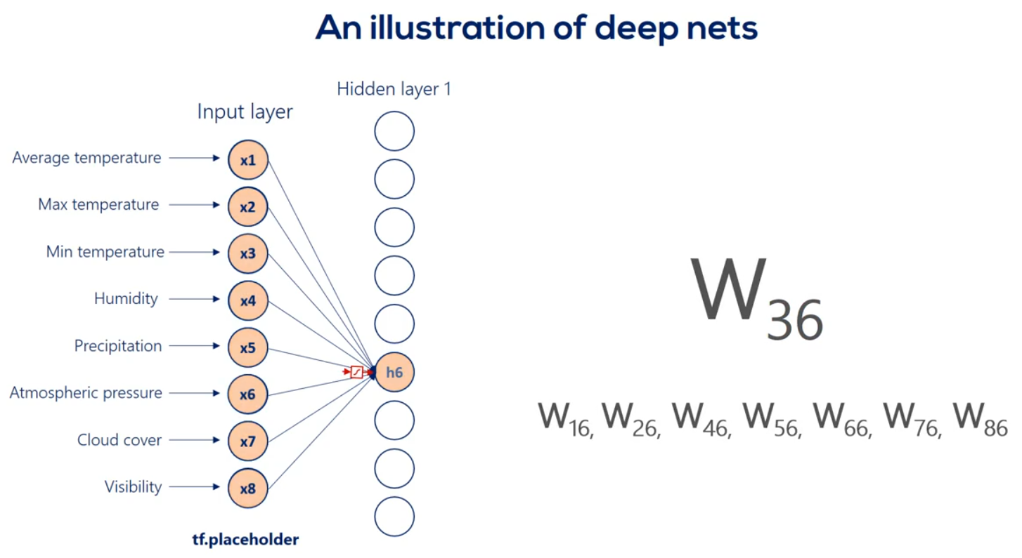
What's Deep Net?

When we have more then one layer, we are talking about neural network.

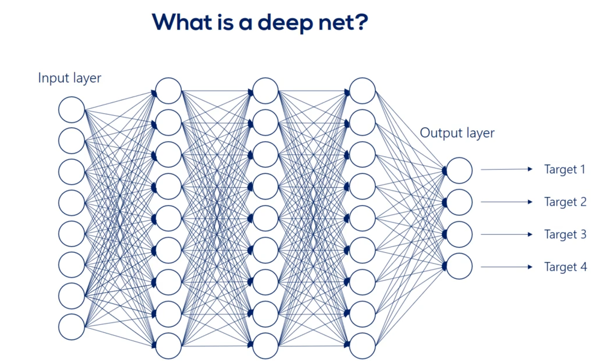
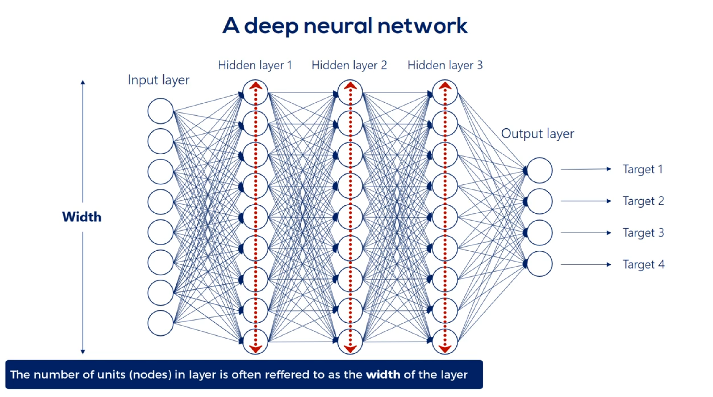
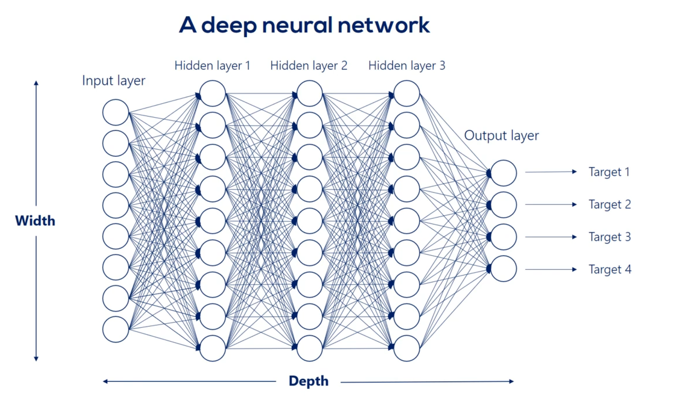
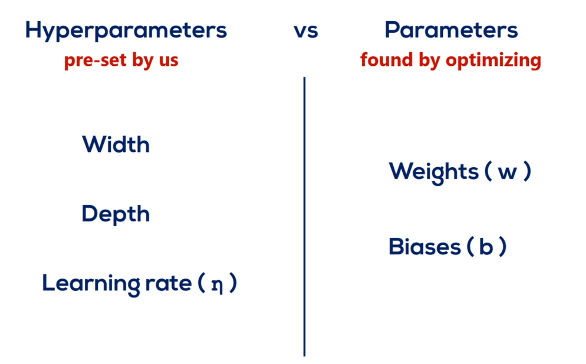
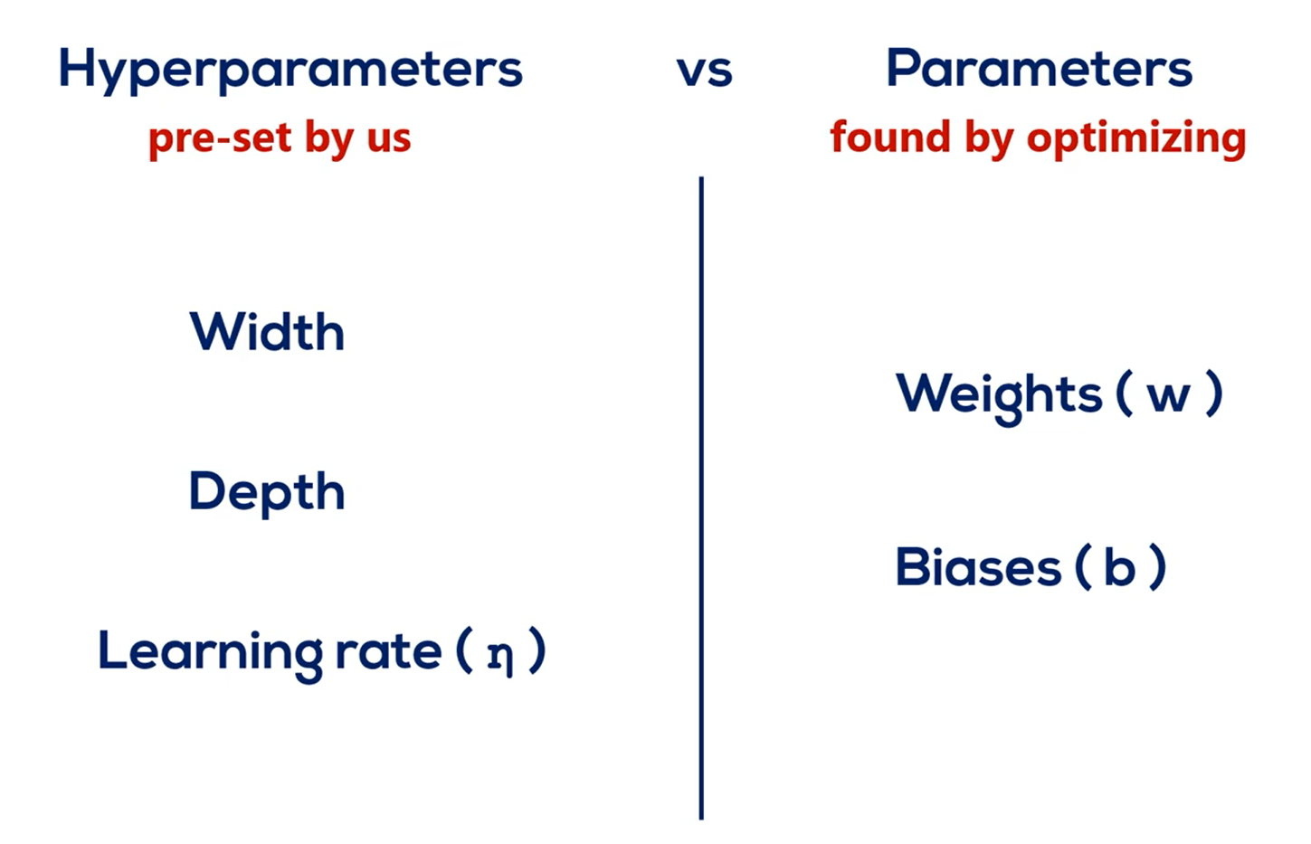
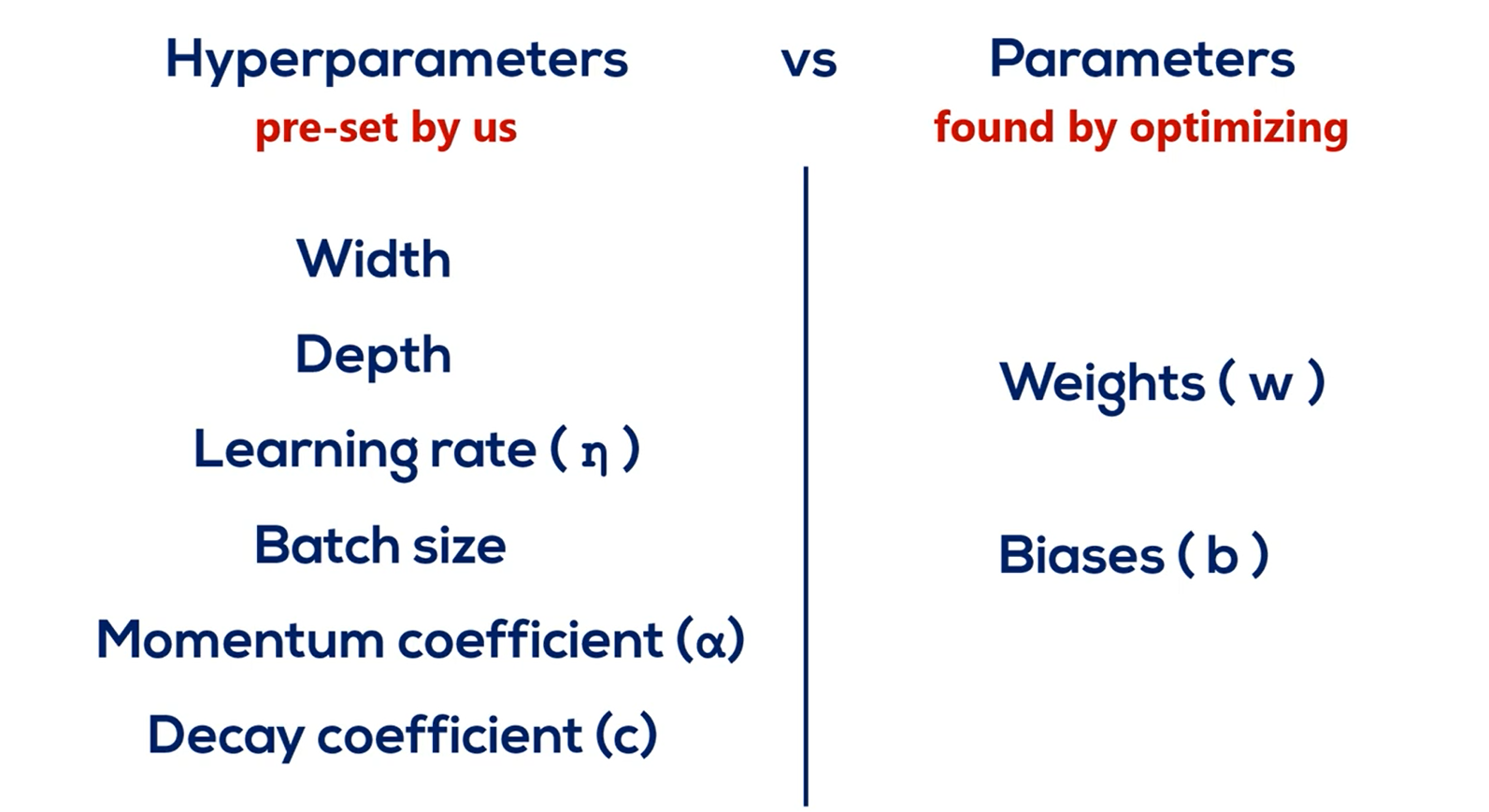
We refer to the width and depth (but not only) as hyperparameters

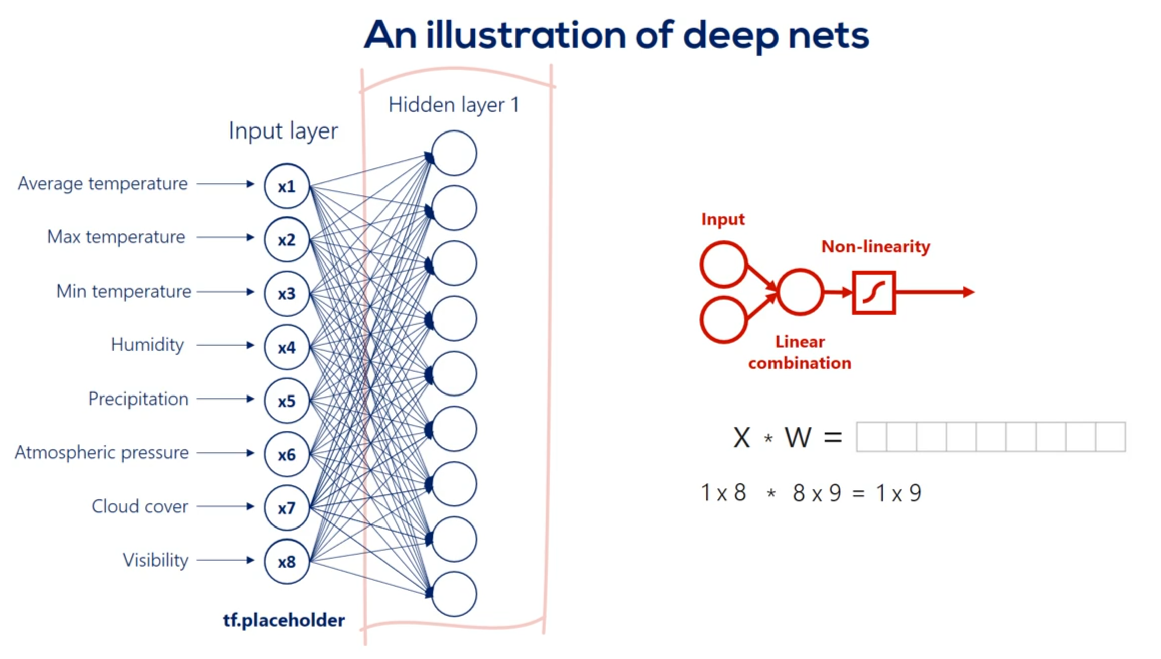
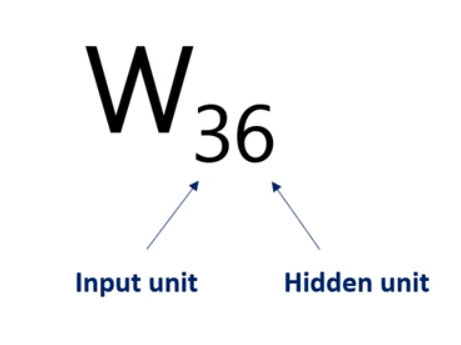
Each arrow represents the mathematical transformation of a certain value

So a certain way is applied then a non-linearity is added know that the non-linearity doesn't change the shape of the expression it only changes its linearity.

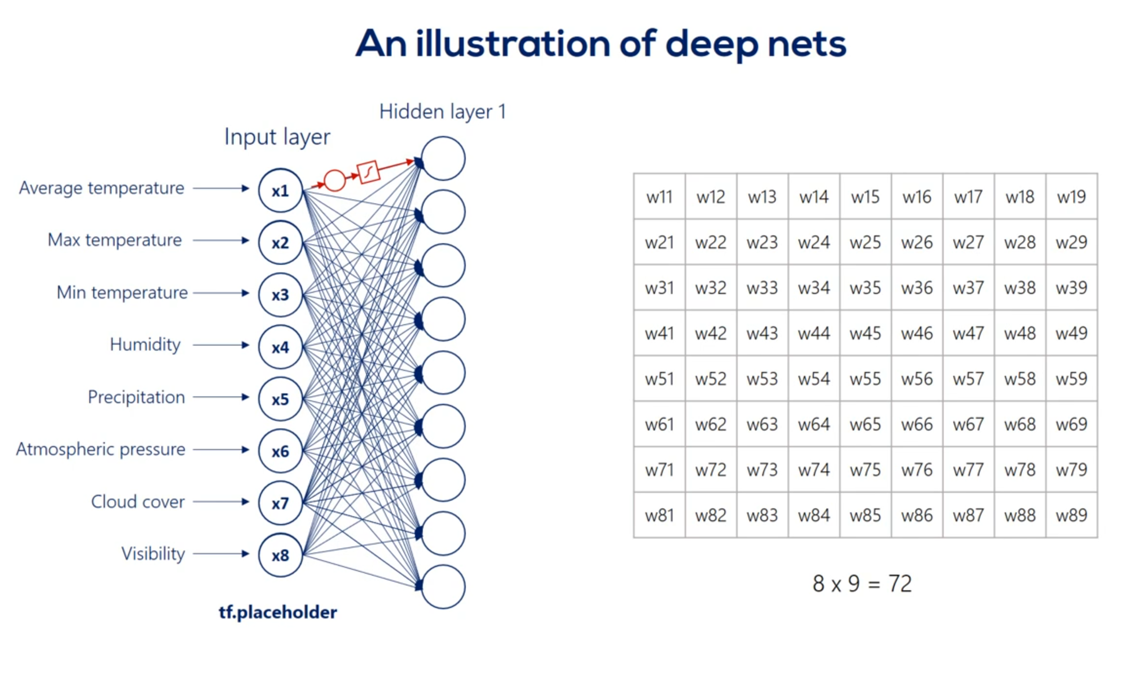
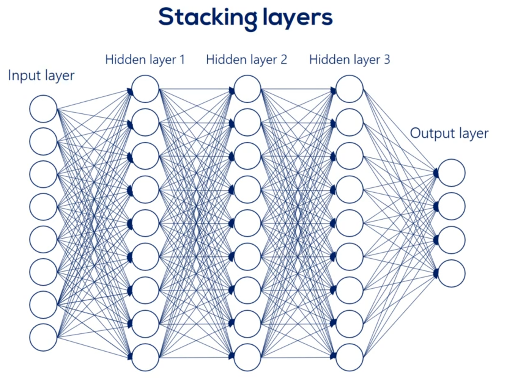
For example weight 3 6 is applied to the third input and is involved in calculating the 6th hidden unit in the same way, Weights 1 6 2 6 and so on until 8 6 all participate in computing the sixth hit and unit. They are linearly combined. And then nonlinearity is added in order to produce the sixth hidden unit in the same way we get each of the other hidden units.

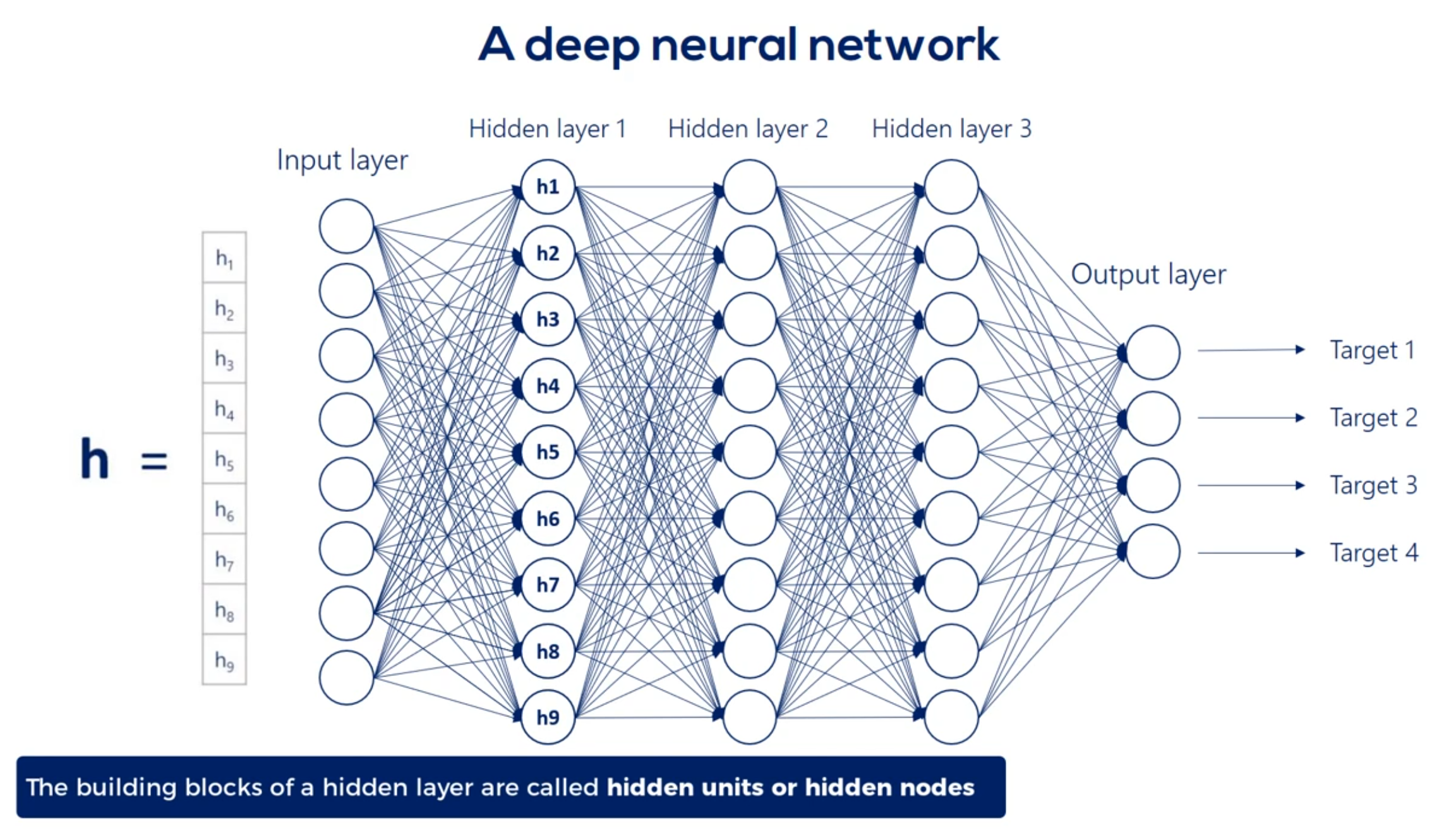
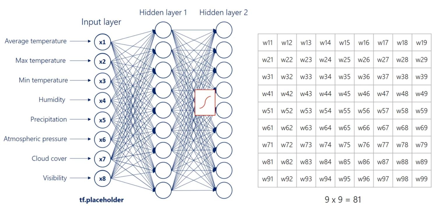
Well then we have the first hit and we're using the same logic we can linearly combine the hidden units and apply a nonlinearity right. Indeed this time though there are nine input hit in units and none output hit in units. Therefore the weights will be contained in a 9 by 9 matrix and there will be 81 arrows. Finally we applied nonlinearity and we reached the second hidden layer. We can go on and on and on like this we can add a hundred hidden layers if we want. That's a question of how deep we want our deep net to be.

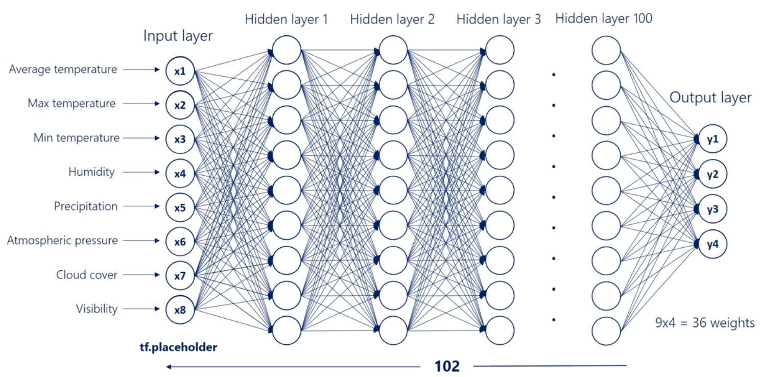
Finally we'll have the last hidden layer when we apply the operation once again we will reach the output layer the output units depend on the number of outputs we would like to have in this picture. There are four. They may be the temperature humidity precipitation and pressure for the next day. To reach this point we will have a nine by four Waite's matrix which refers to 36 arrows or 36 weights exactly what we expected.

Why do we need non-linearities

All right as before our optimization goal is finding values for major cities that would allow us to convert inputs into correct outputs as best as we can. This time though we are not using a single linear model but a complex infrastructure with a much higher probability of delivering a meaningful result.

We said non-linearities are needed so we can represent more complicated relationships. While that is true it isn't the full picture an important consequence of including non-linearities is the ability to stack Layers stacking layers is the process of placing one layer after the other in a meaningful way. Remember that it's fundamental.

We cannot stack layers when we only have linear relationships.

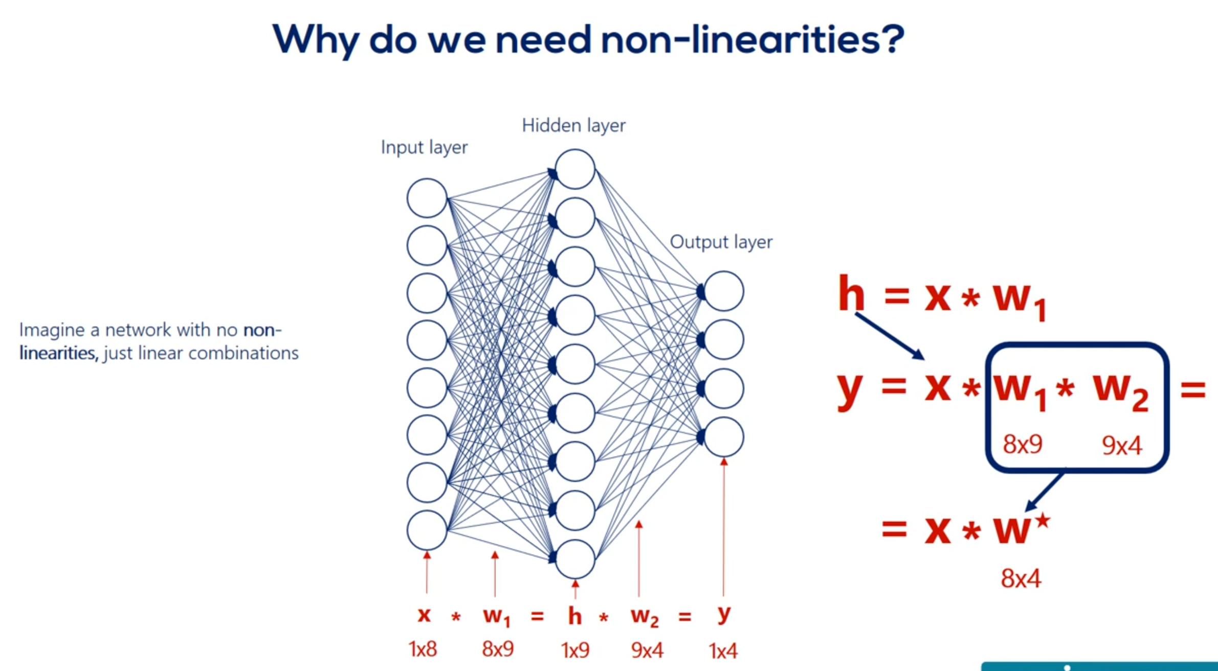
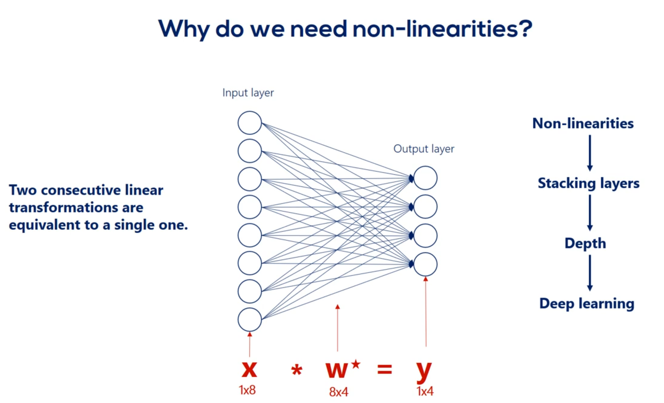
The point we will make is that we cannot stack Lears when we have only linear relationships. Let's prove it. Imagine we have a single hidden layer and there are no non-linearities. So our picture looks this way. There are eight input nodes nine head and nodes in the hidden layer and four output nodes. Therefore we have an eight by nine Waites matrix. When your relationship between the input layer and the hidden layer Let's call this matrix W. one. The hidden units age according to the linear model H is equal to x times w 1. Let's ignore the biases for a while. So our hidden units are summarized in the matrix H with a shape of one by nine. Now let's get to the output layer from the hidden layer once again according to the linear model Y is equal to h times W2 we have W2 as these weights are different. We already know the H matrix is equal to x times. W1 Right. Let's replace h in this equation Y is equal to x times w 1 times. W2 but w 1 and w 2 can be multiplied right. What we get is a combined matrix W star with dimensions 8 by 4 well then our deep net can be simplified into a linear model which looks this way y equals x times w star knowing that we realize the hidden layer is completely useless in this case. We can just train this simple linear model and we would get the same result in mathematics. This seems like an obvious fact but in machine learning it is not so clear from the beginning. The two consecutive linear transformations are equivalent to a single one. Even if we add 100 layers the problem would be simplified to a single transformation. That is the reason we need non-linearities. Without them stacking layers one after the other is meaningless and without stacking layers we will have no depth. What's more with no depth. Each and every problem will equal the simple linear example we did earlier. And many practitioners would tell you it was borderline machine learning. All right let's summarize in one sentence.

You have deep nets and find complex relationships through arbitrary functions. We need non-linearities.

Point taken.

Non-linearities are also called activation functions. Henceforth that's how we will refer to them activation functions transform inputs into outputs of a different kind.

Activation functions

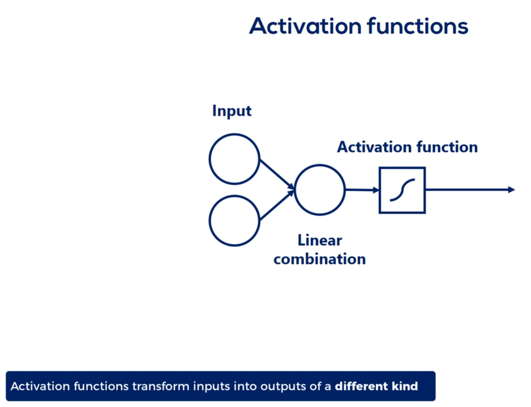
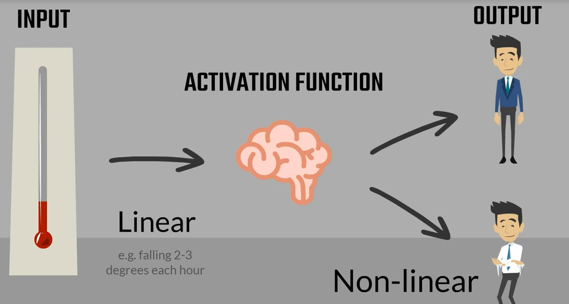
Think about the temperature outside. I assume you wake up and the sun is shining. So you put on some light clothes you go out and feel warm and comfortable. You carry your jacket in your hands in the afternoon the temperature starts decreasing. Initially you don't feel a difference at some point though your brain says it's getting cold. You listen to your brain and put on your jacket the input you got was the change in the temperature the activation function transformed this input into an action put on the jacket or continue carrying it. This is also the output after the transformation. It is a binary variable jacket or no jacket. That's the basic logic behind nonlinearities the change in the temperature was following a linear model

as it was steadily decreasing the activation function transformed this relationship into an output linked to the temperature but was of a different kind

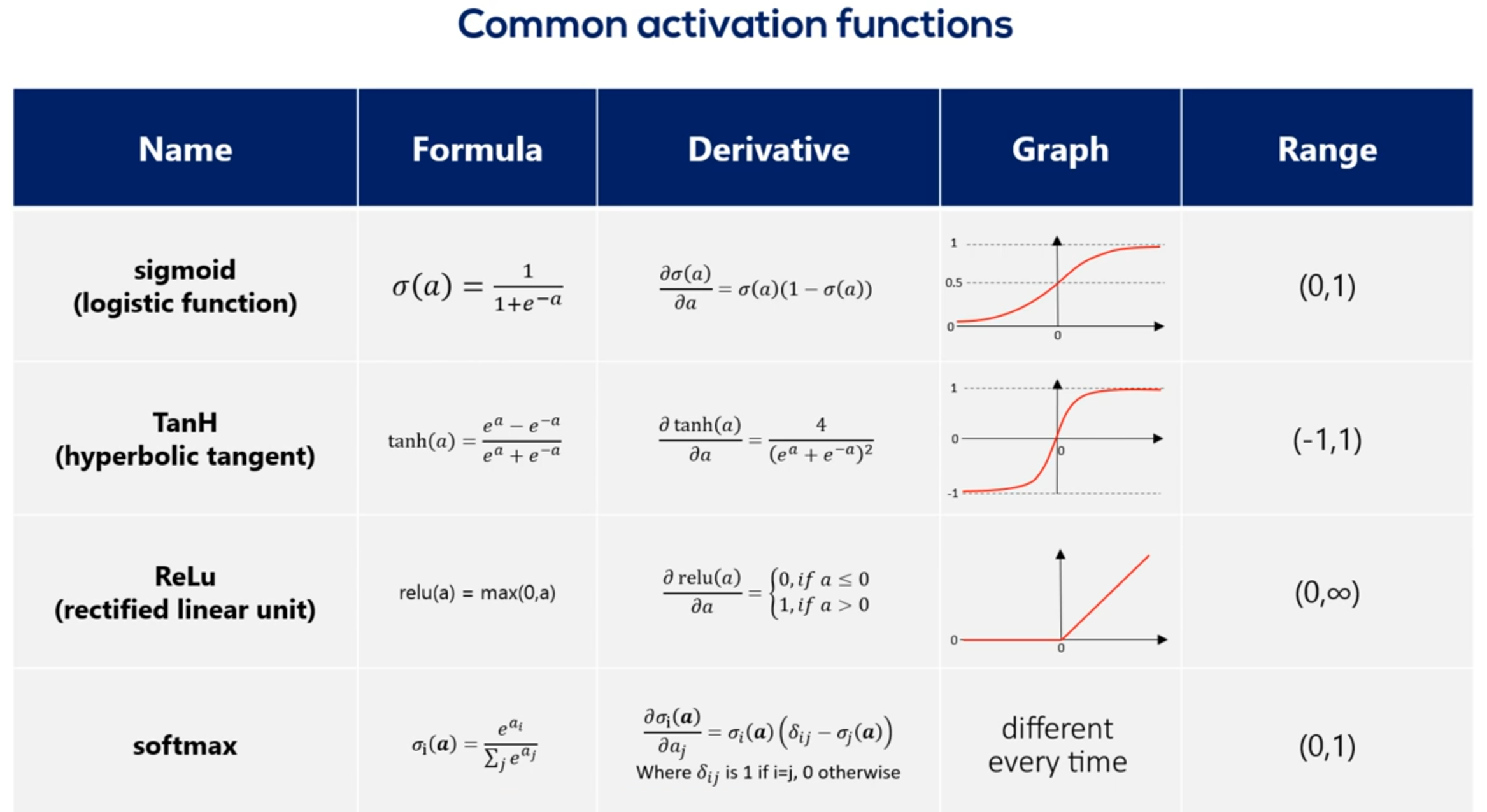
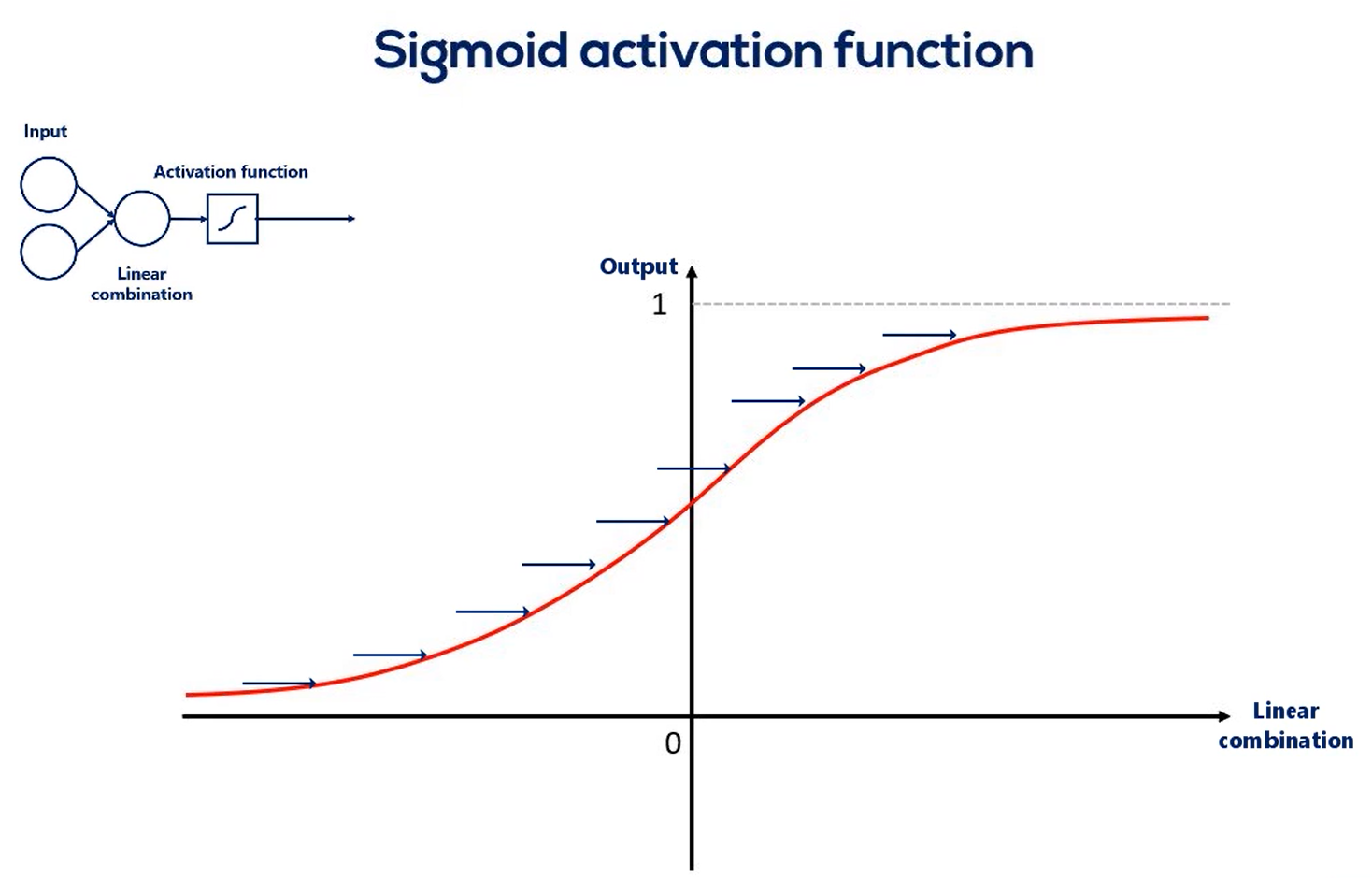
its derivative as you may recall the derivative is an essential part of the gradient descent. Naturally when we work with tenths or flow we won't need to calculate the derivative as tenths or flow. Does that automatically Anyhow the purpose of this lesson is understanding these functions. There are graphs and ranges in a way that would allow us to acquire intuition about the way they behave. Here's the functions graph. And finally we have it's range. Once we have applied the sigmoid as an activator all the outputs will be contained in the range from 0 to 1. So the output is somewhat standardized. All right here are the other three common activators the Tench also known as the hyperbolic tangent. The real Lu aka the rectified linear unit and the soft Max activator you can see their formulas derivatives graphs and ranges. The saaf next graph is not missing. The reason we don't have it here is that it is different every time. Pause this video for a while and examine the table in more detail. You can also find this table in the course notes. So all these functions are activators right. What makes them similar. Well let's look at their graphs all Armano tonic continuous and differentiable. These are important properties needed for the optimization process as we are not there yet. We will leave this issue for later.

Before we conclude I would like to make this remark. Activation functions are also called transfer functions because of the transformation properties. The two terms are used interchangeably in machine learning context but have differences in other fields. Therefore to avoid confusion we will stick to the term activation functions.

Softmax function

Let's continue exploring this table which contains mostly Greek letters we said the soft max function has no definite graph y so while this function is different if we take a careful look at its formula we would see the key difference between this function and the other is it takes an argument the whole vector A instead of individual elements. So the self max function is equal to the exponential of the element at position. I divided by the sum of the exponentials of all elements of the vector. So while the other activation functions get an input value and transform it regardless of the other elements the SAAF Max considers the information about the whole set of numbers we have.

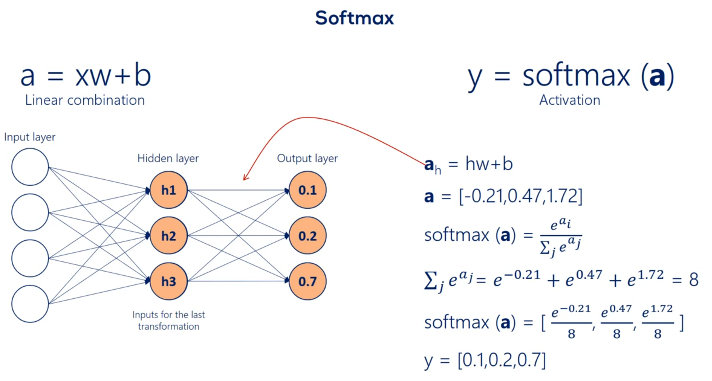
A key aspect of the soft Max transformation is that the values it outputs are in the range from 0 to 1. There is some is exactly 1 What else has such a property. Probabilities Yes probabilities indeed. The point of the soft Max transformation is to transform a bunch of arbitrarily large or small numbers that come out of previous layers and fit them into a valid probability distribution. This is extremely important and useful.

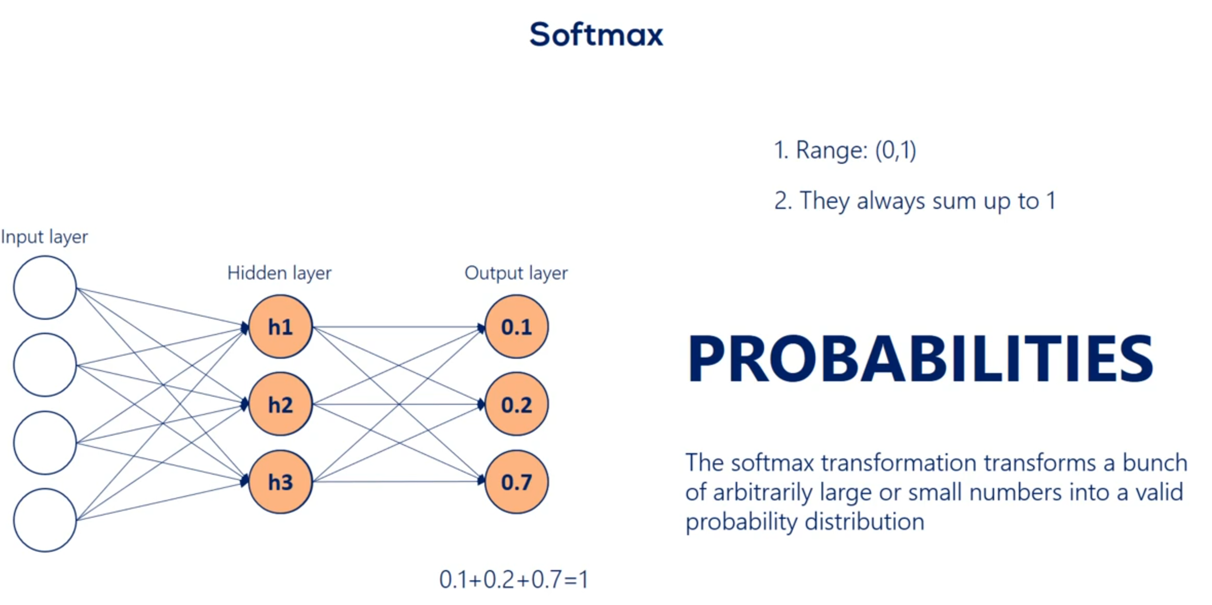
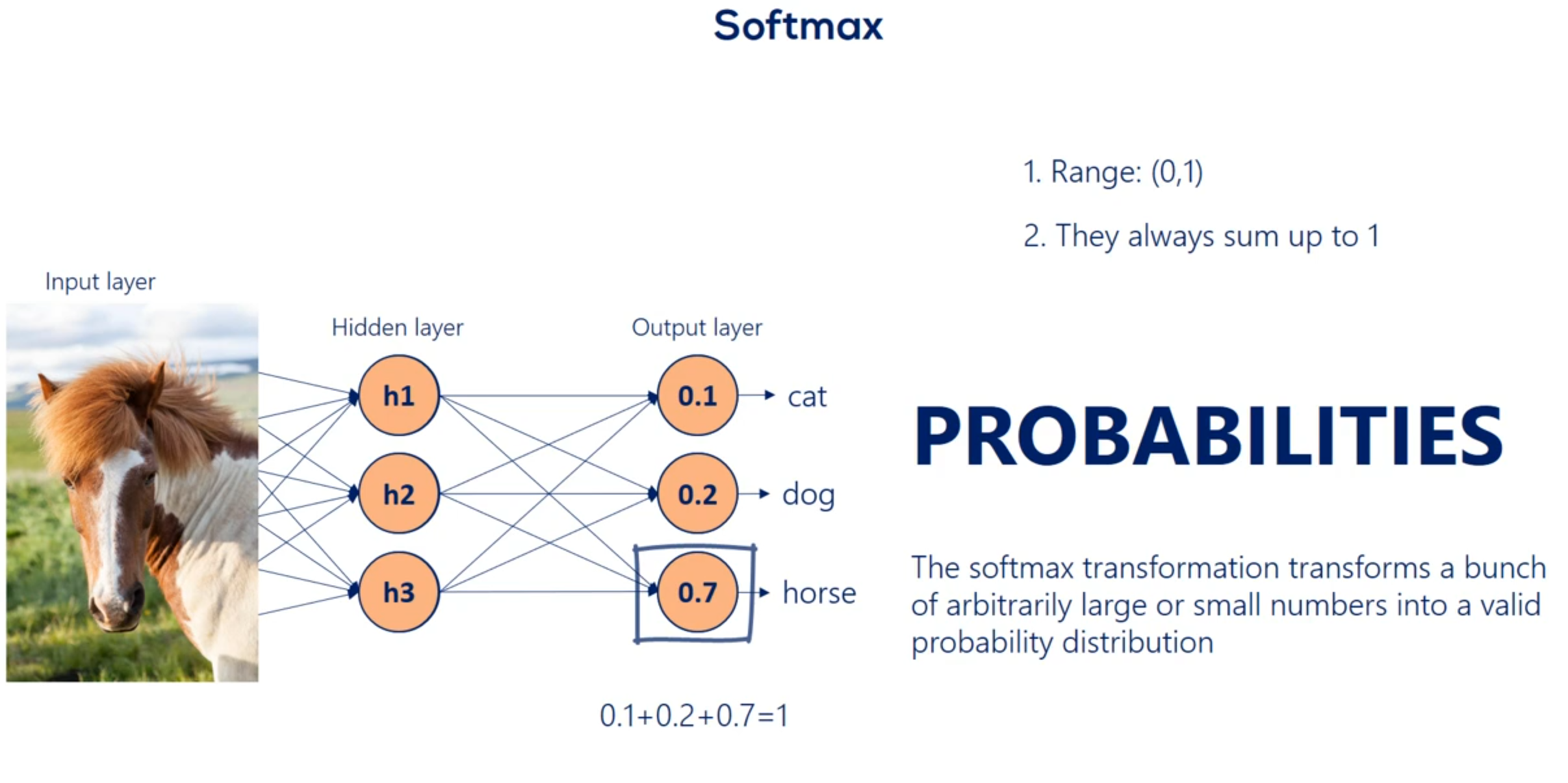
Remember our example with cats dogs and horses we saw earlier. One photo was described by a vector containing 0.1 0.2 and 0.7. We promise we will tell you how to do that. Well that's how through a soft Max transformation we kept our promise now that we know we are talking about probabilities we can comfortably say we are 70 percent certain the image is a picture of a horse. This makes everything so intuitive and useful that the SAAF next activation is often used as the activation of the final output layer and classification problems. So no matter what happens before the final output of the algorithm is a probability distribution.

Backpropagation

First I'd like to recap what we know so far we've seen and understood the logic of how layers are stacked.

We've also explored a few activation functions and spent extra time showing they are central to the concept of stacking layers.

Moreover by now we have said 100 times that the training process consists of updating parameters through the gradient descent for optimizing the objective function.

In supervised learning the process of optimization consisted of minimizing the loss.

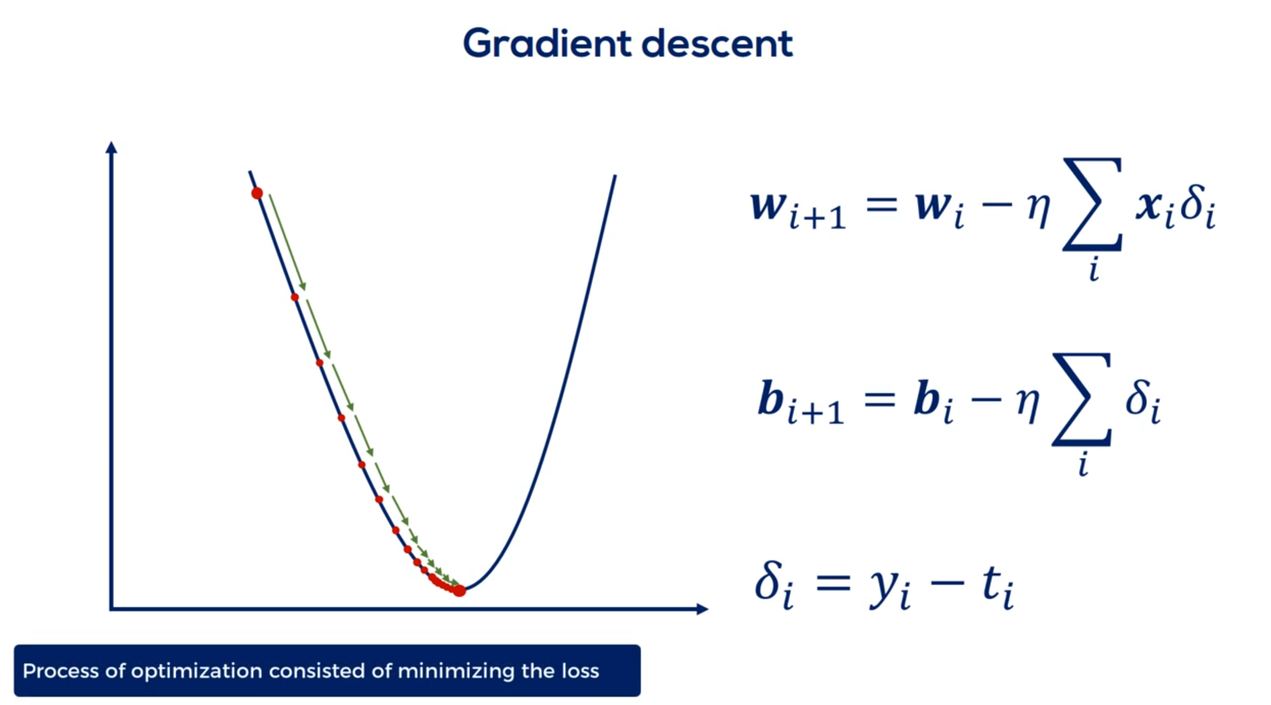
Our updates were directly related to the partial derivatives of the loss and indirectly related to the

errors or deltas as we called them.

Let me remind you that the Deltas were the differences between the targets and the outputs.

All right as we will see later deltas for the hidden layers are trickier to define. Still they have a similar meaning.

The procedure for calculating them is called back propagation of errors having these deltas allows us to vary parameters using the familiar update rule.

Let's start from the other side of the coin forward propagation

Forward propagation is the process of pushing inputs through the net.

At the end of each epoch the obtained outputs are compared to the targets to form the errors.

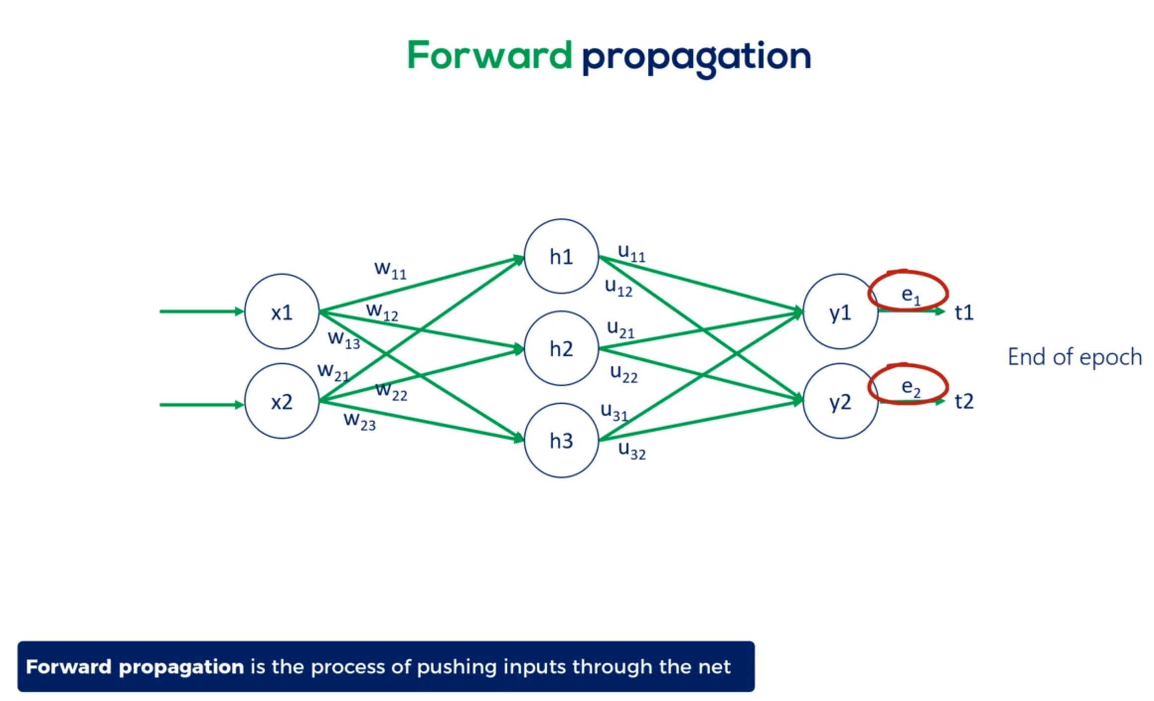
Then we back propagate through partial derivatives and change each parameter so errors at the next epoch are minimized.

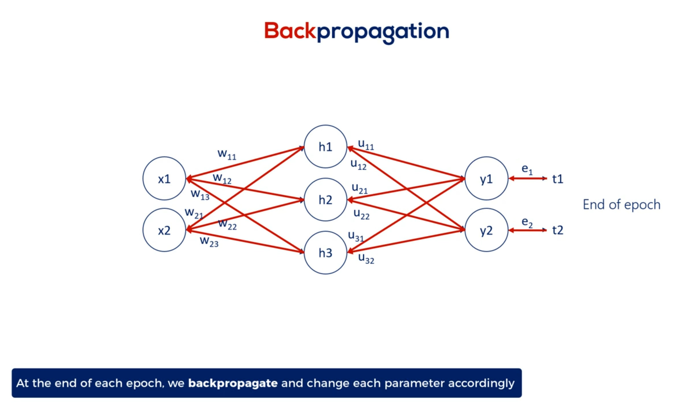
For the minimal example the back propagation consisted of a single step, aligning the weights, given the errors we obtained.

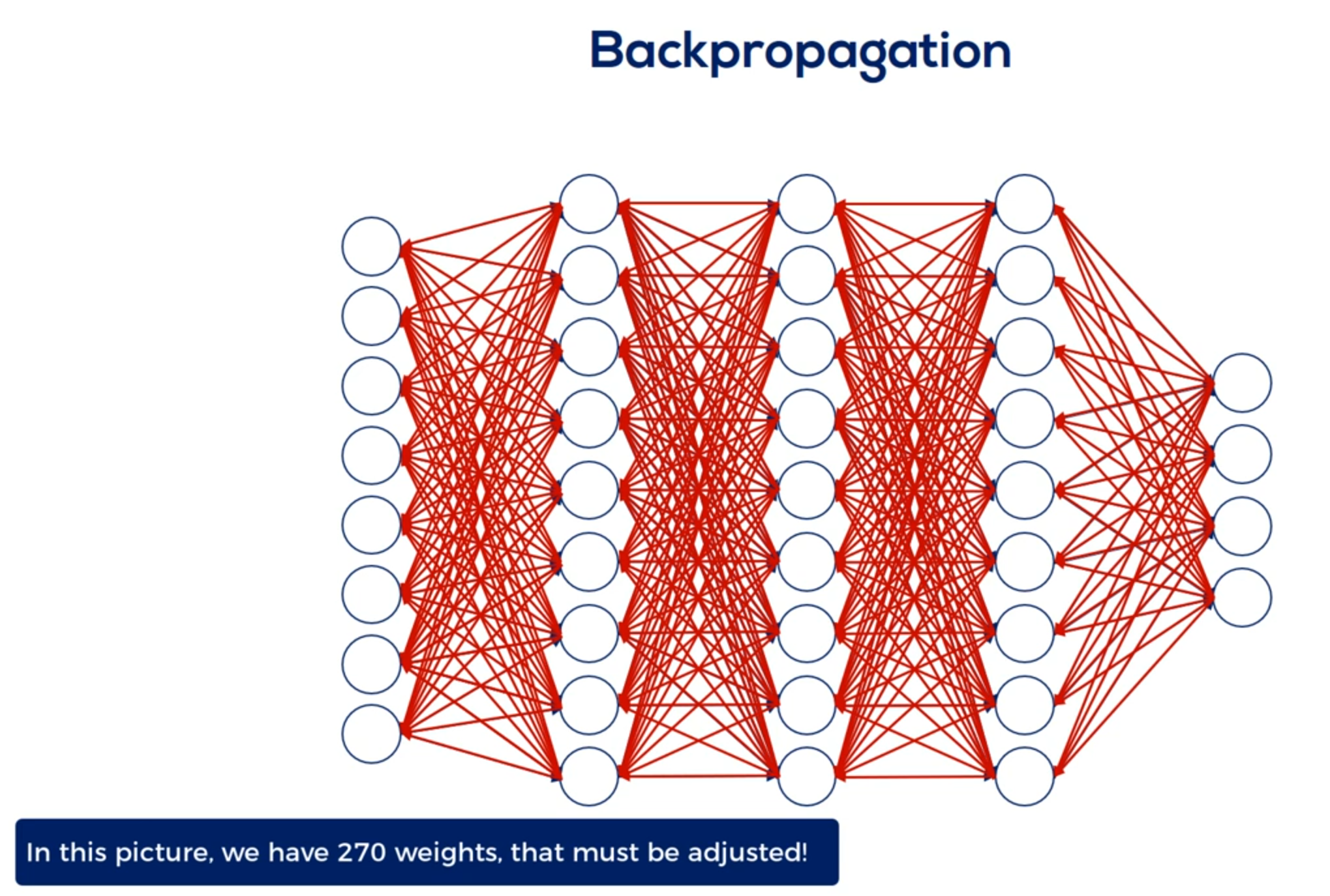
Here's where it gets a little tricky when we have a deep net. We must update all the weights related to the input layer and the hidden layers. For example in this famous picture we have 270 weights and yes this means we had to manually draw all 270 arrows you see here.

So updating all 270 weights is a big deal.

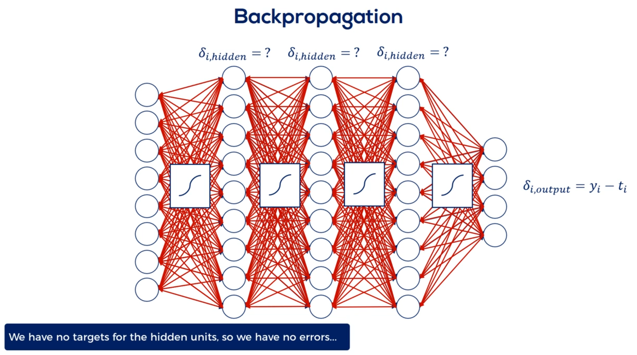
But wait. We also introduced activation functions. This means we have to update the weights accordingly. Considering the use nonlinearities and their derivatives.

Finally to update the weights we must compare the outputs to the targets. This is done for each layer but we have no targets for the hidden units. We don't know the errors So how do we update the weights. That's what back propagation is all about. We must arrive the appropriate updates as if we had targets.

Now the way academics solve this issue is through errors. The main point is that we can trace the contribution of each unit hit or not to the error of the output.

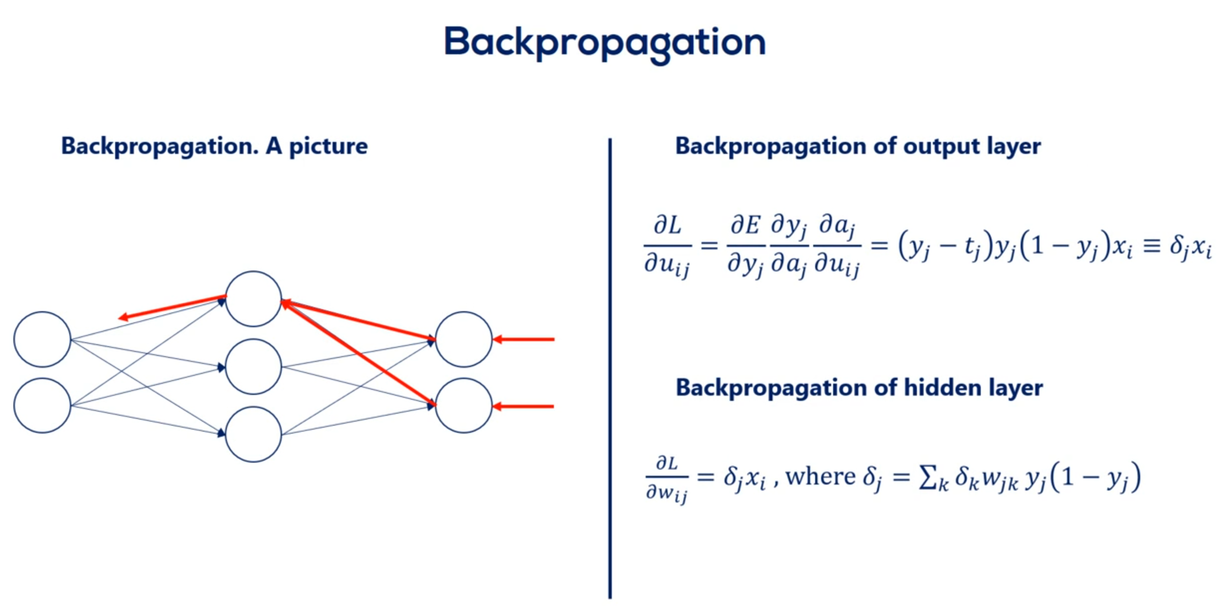
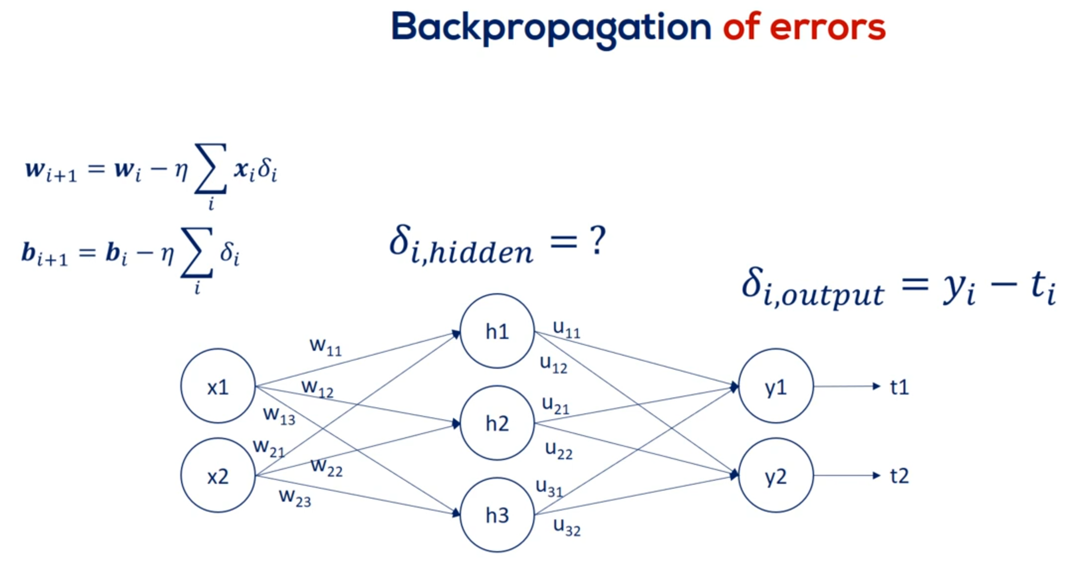
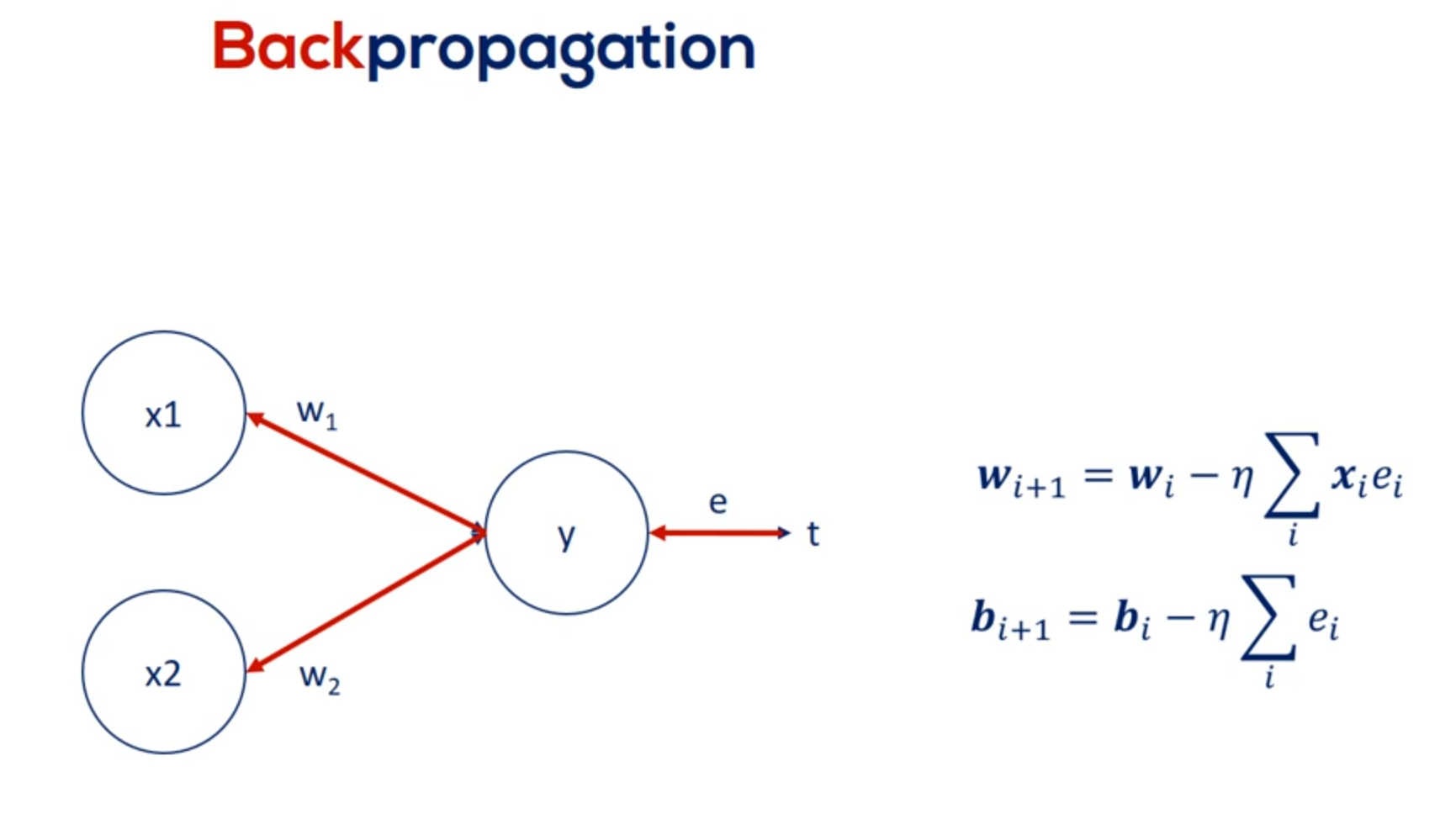
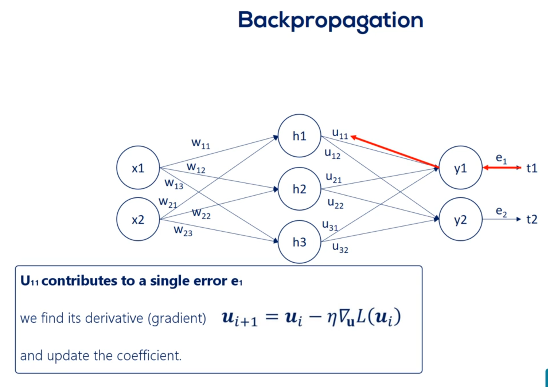
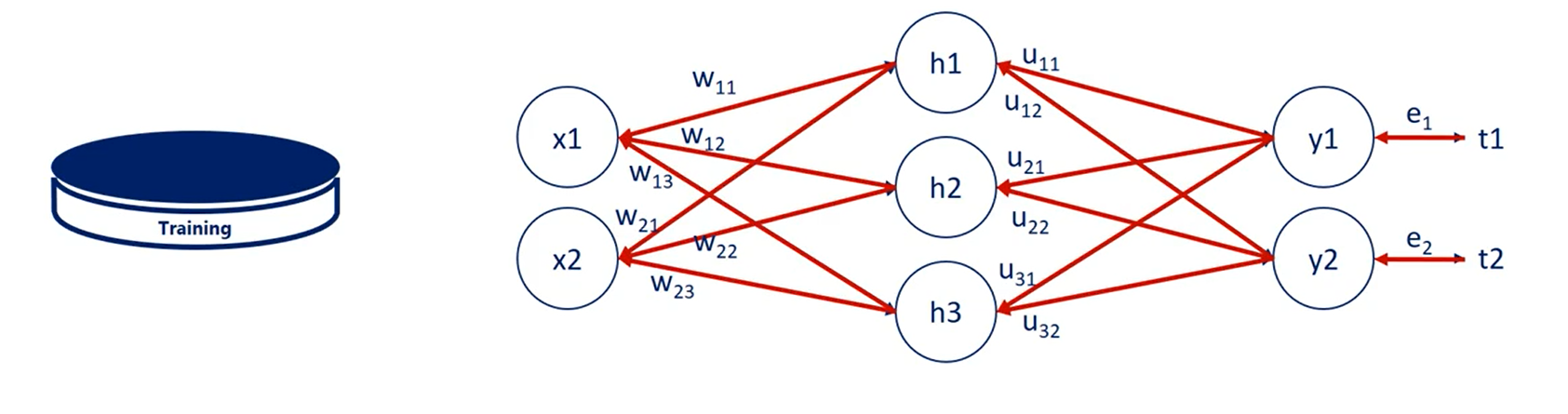
OK great let's look at the schematic illustration of back propagation shown here our net is quite simple.

It has a single hidden layer.

Each node is labeled.

So we have inputs x 1 and x 2 hidden layer units output layer units. Why one in y2 two. And finally the targets T1 and T2.

The weights are w 1 1 w 1 2 w 1 3 w 2 1 w 2 2 and W 2 3 for the first part of the net. For the second part we named them you 1 1 you 1 2 you 2 1 you 2 2 3 1 and you 3 2. So we can differentiate between the two types of weights.

That's very important.

We know the error associated with Y 1 and y to as it depends on known targets. So let's call the two errors. E 1 and 2.

Based on them we can adjust the weights labeled with you. Each U contributes to a single error.

For example you 1 1 contributes to e 1.

Then we find its derivative and update the coefficient. Nothing new here.

Now let's examine w 1 1 . Helped us predict h1 But then we needed h1 to calculate y1 in y2. Thus it played a role in determining both errors. e1 and e2.

So while u11 contributes to a single error w11 contributes to both errors. Therefore it's adjustment rule must be different.

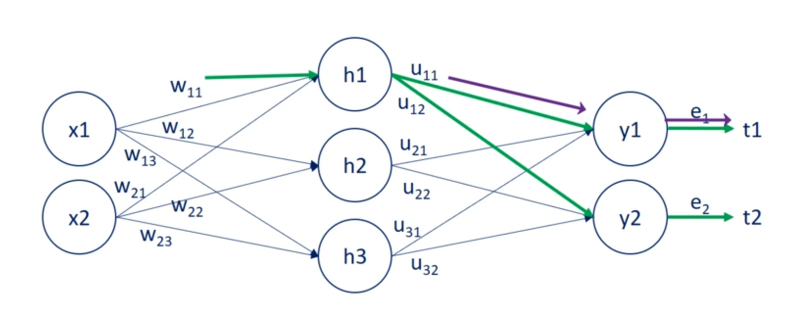
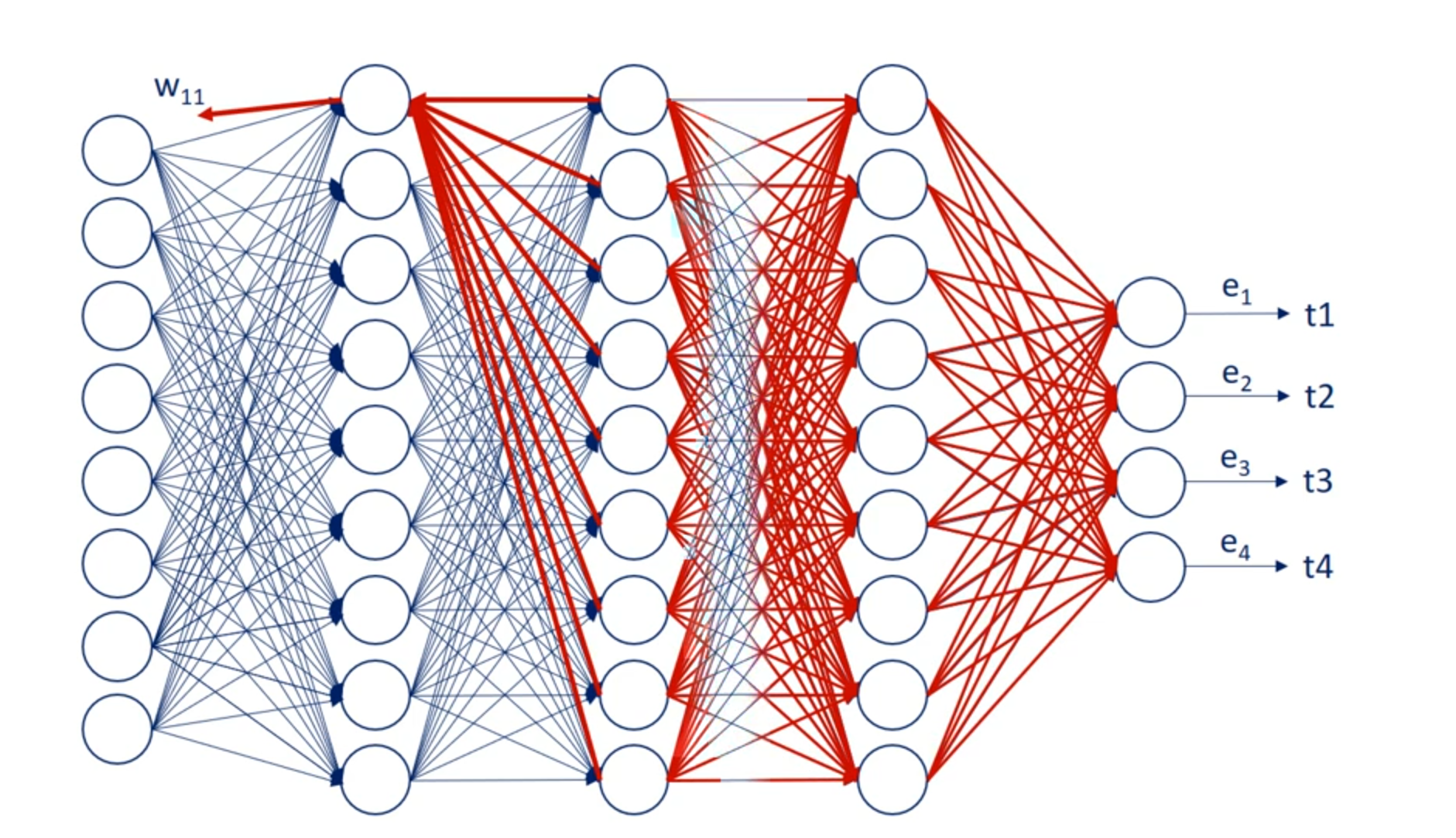
The solution to this problem is to take the errors and back propagate them through the net using the weights.

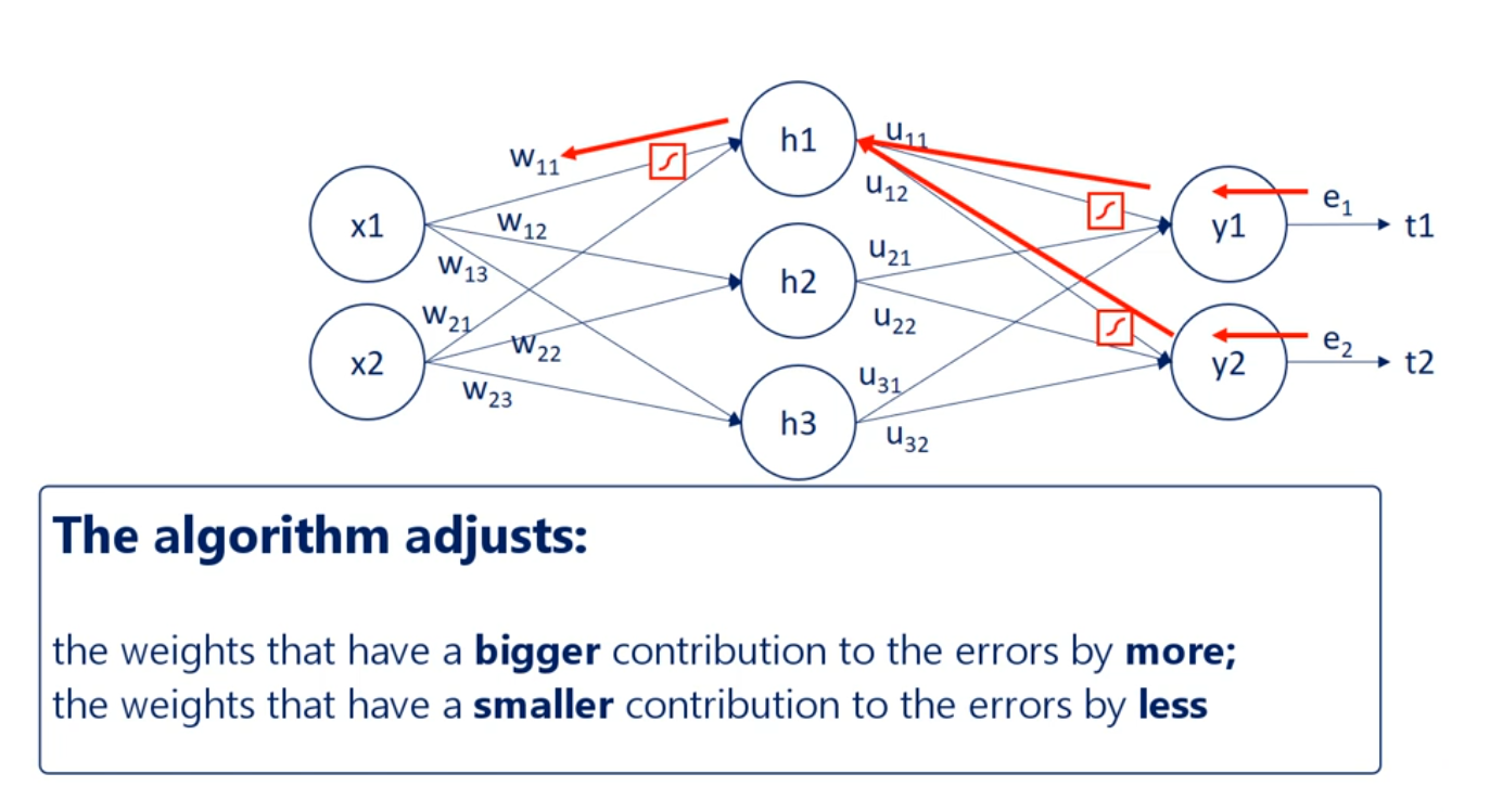
Knowing the u weights we can measure the contribution of each hit in unit to the respective errors.

Then once we found out the contribution of each hit in unit to the respective errors we can update the W weights.

So essentially through back propagation the algorithm identifies which weights lead to which errors then it adjusts the weights that have a bigger contribution to the errors by more than the weights with a smaller contribution.

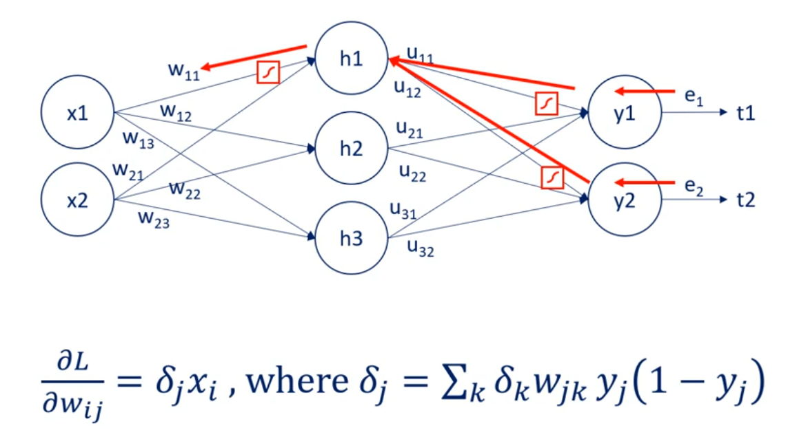
A big problem arises when we must also consider the activation functions. They introduce additional complexity to this process.

Linear your contributions are easy but non-linear ones are tougher. Emergent back propagating in our introductory net. Once you understand it, it seems very simple.

While pictorially straightforward mathematically it is rough to say the least.

That is why back propagation is one of the biggest challenges for the speed of an algorithm.

WARNING

Continue on Chapter 8 of the desktop course

Practical lessons on chapters 12 and 13

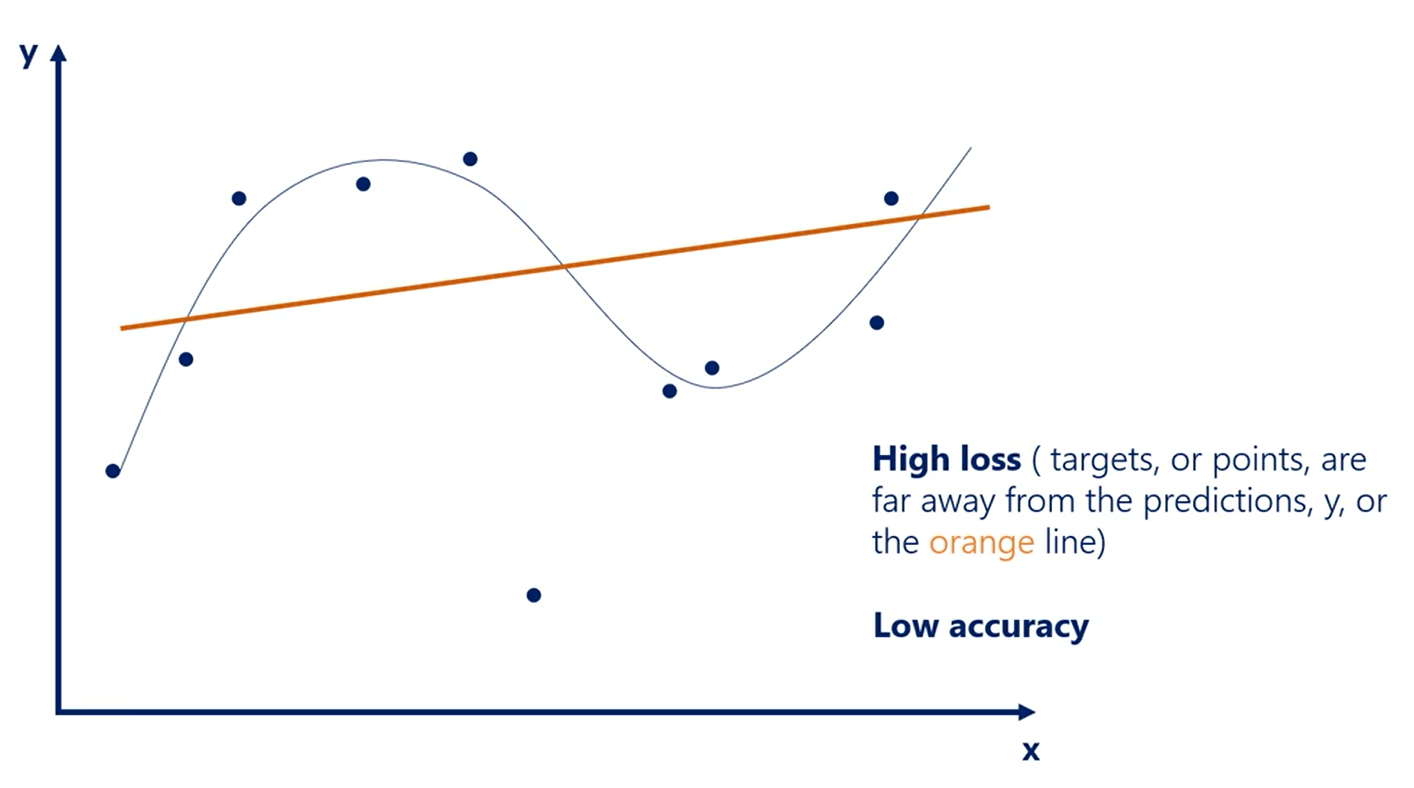
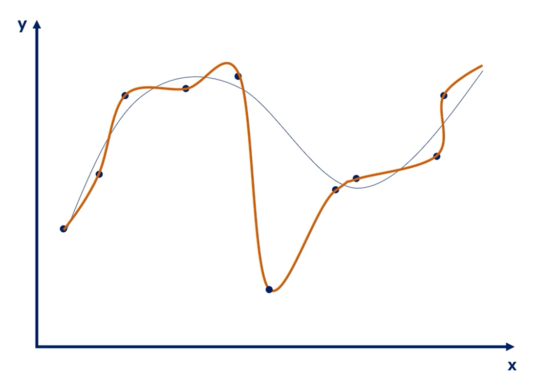
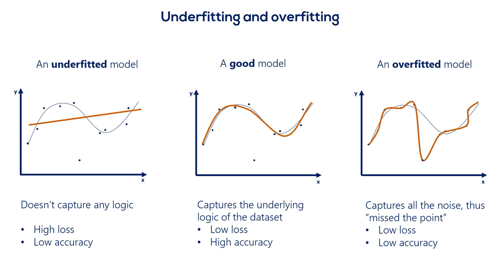
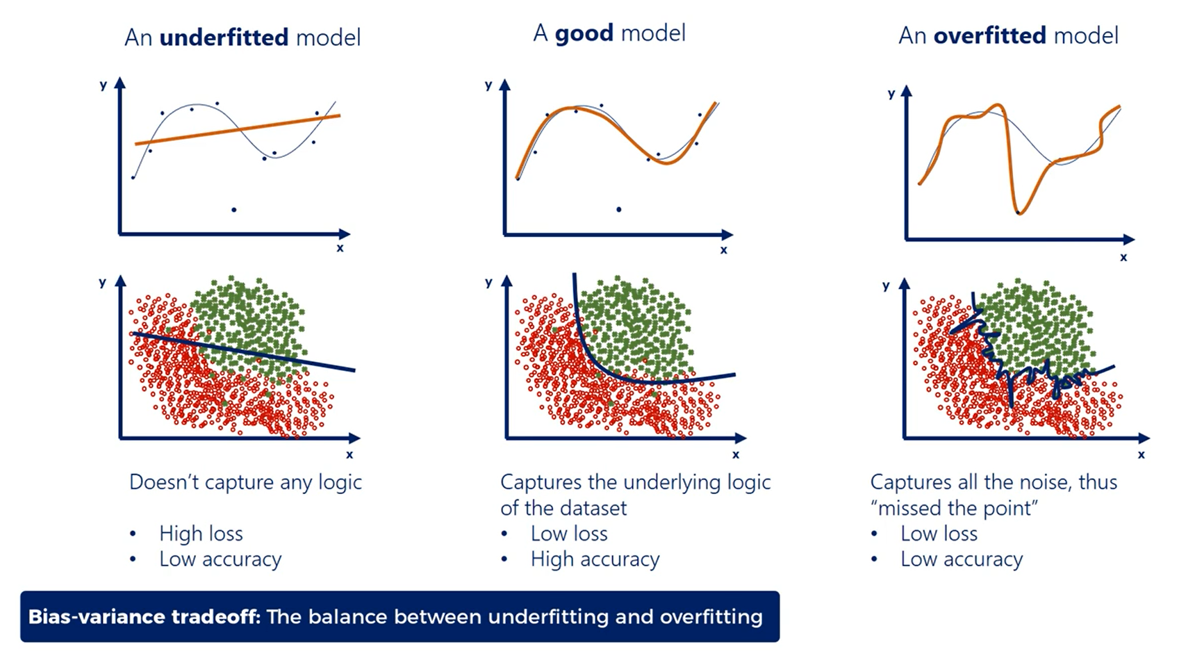
Overfitting

Underfitting	Overfitting
The model has not capture the underlying logic of the data	Our training has focused on the particular training set so much, it has "missed the point"

A good model:

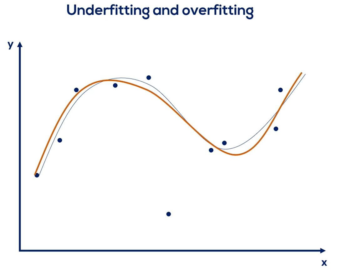
Underfitted Model:

Overfitted Model:

Comparison:

Overfitting - A classification example

Preventing Overfitting

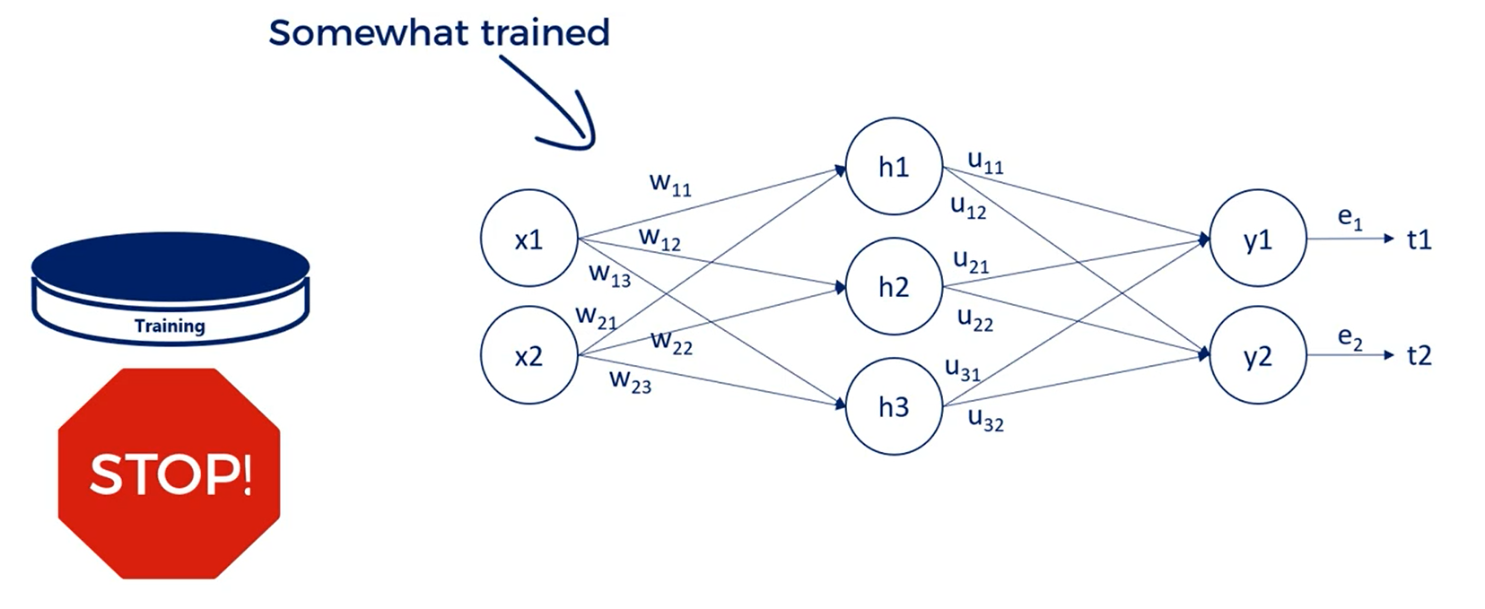
Training and Validation

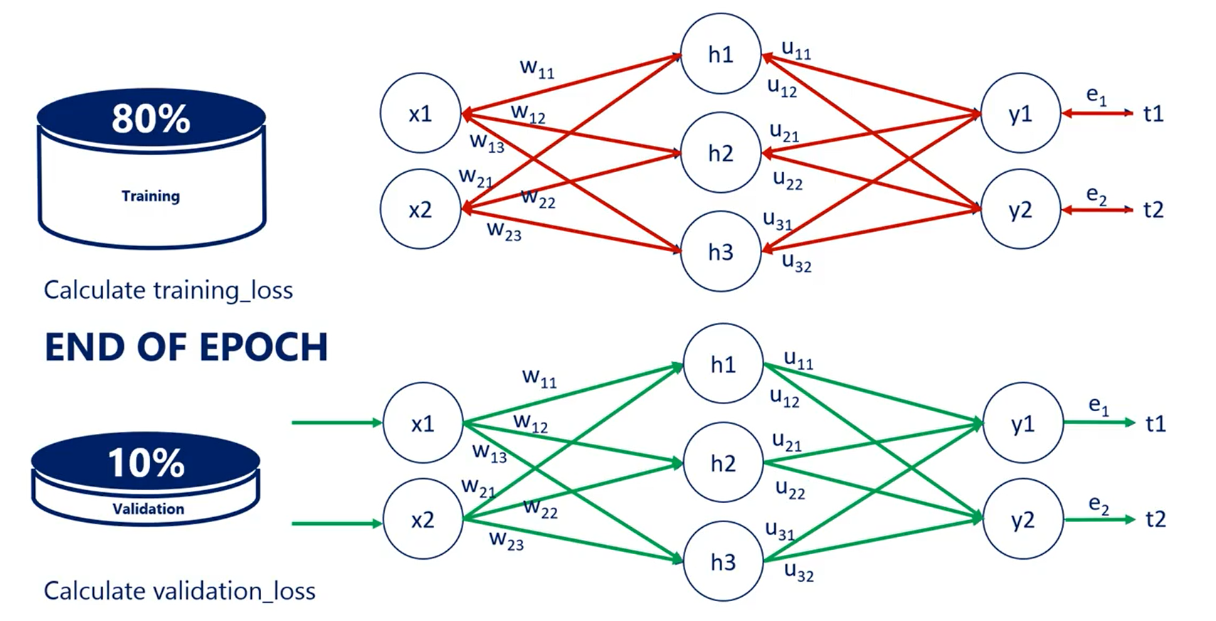
All the training is done on the training set.

In other words we update the weights for the training so only every once in a while we stop training for a bit. At this point the model is somewhat trained.

What we do next is take the model and apply it to the validation data set. This time we just run it without updating the weights so we only propagate forward not backward.

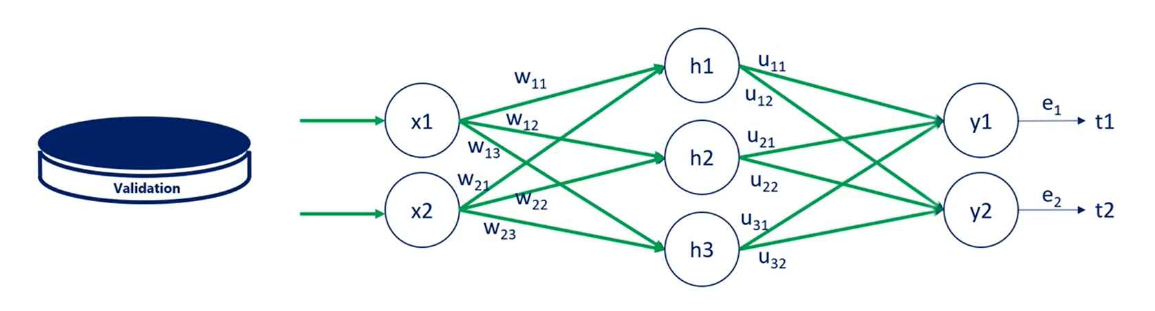
In other words we just calculate its loss function on average the last function calculated for the validation set should be the same as the one of the training set.

This is logical as the training and validation sets were extracted from the same initial dataset containing the same perceived dependencies.

Normally, we would perform this operation many times in the process of creating a good machine learning algorithm.

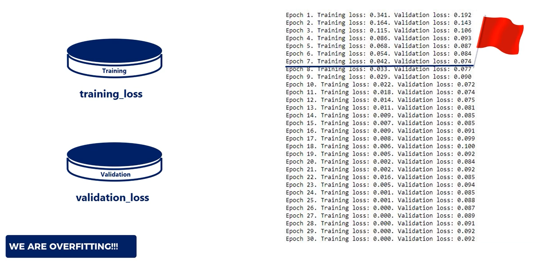
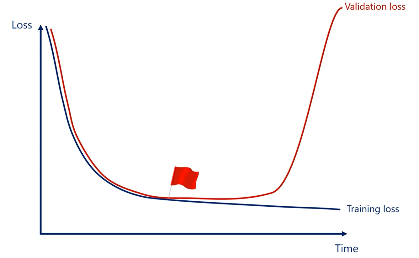
The two last functions we calculate are referred to as training loss and validation loss and because the data in the training is trained using the gradient descent, each subsequent loss will be lower or equal to the previous one. That's how gradient descent works by definition, so we are sure that treating loss is being minimized.

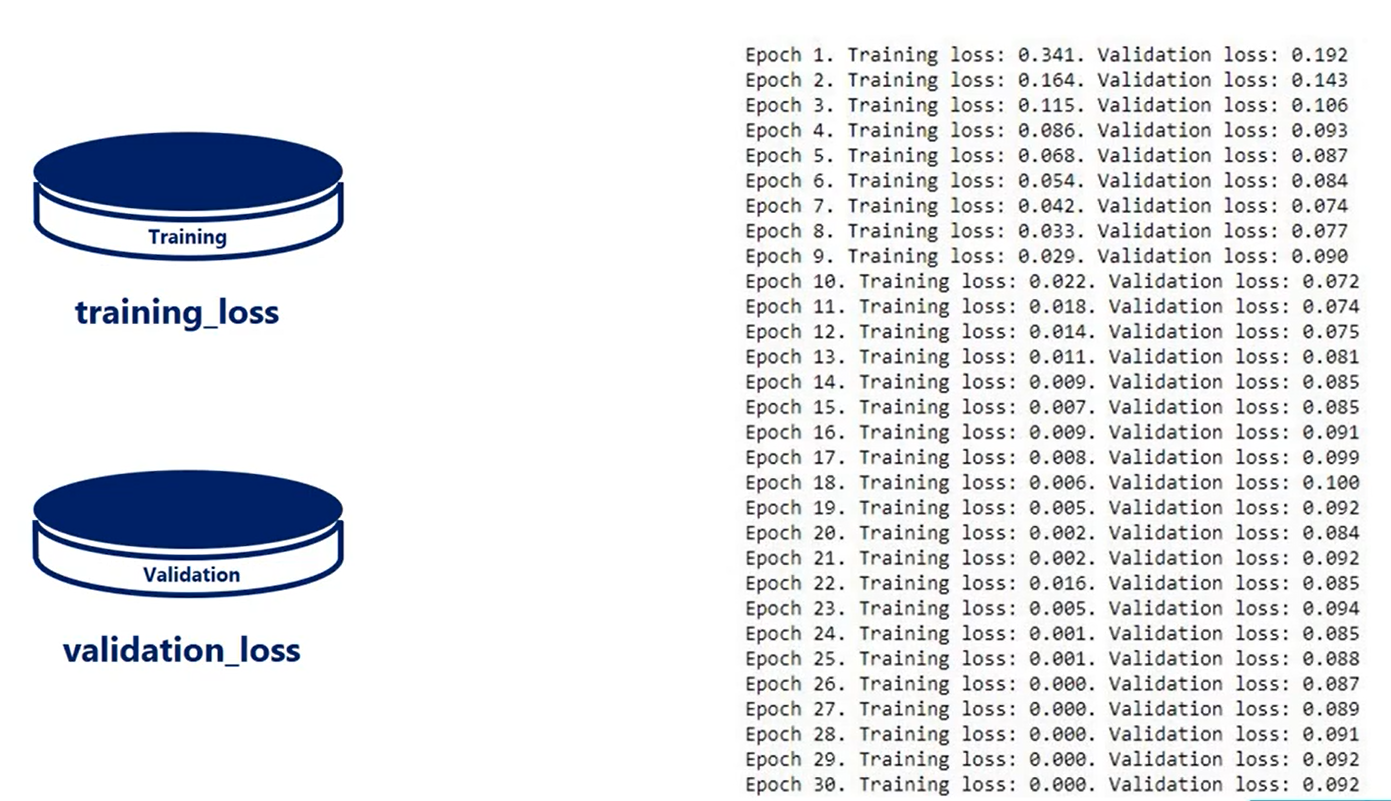
That's where the validation loss comes in play at some point the validation loss could start increasing. That's a red flag. We are overfitting we are getting better at predicting the training set but we are moving away from the overall logic data. At this point we should stop training the model.

WARNING

It is extremely important that the model is not trained on validation samples.

This will eliminate the whole purpose of the above mentioned process.

The training set and the validation set should be separate without overlapping each other.

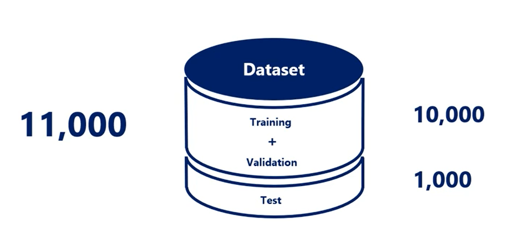
Training, Validation and Test

We introduce the validation data set. In addition, we said we want to divide the initial dataset into three parts.

Training, validation and Test.

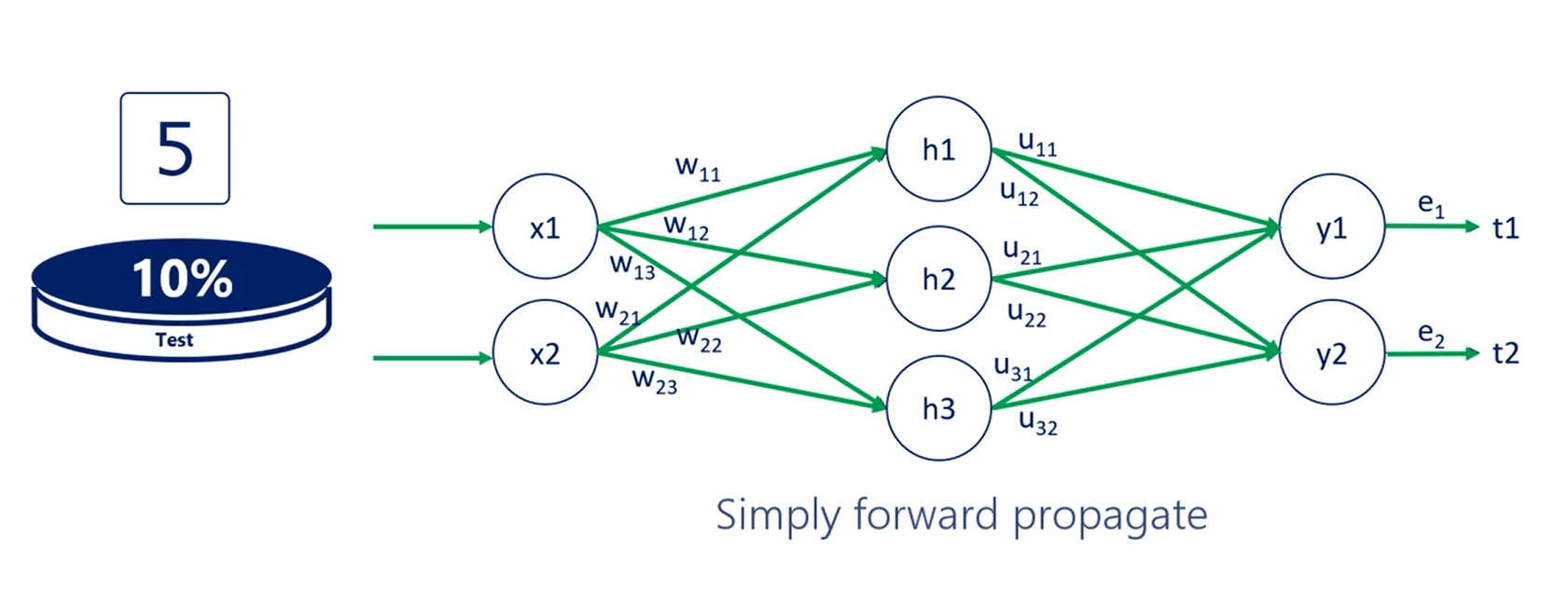
After we have trimmed the model and validated it, it is time to measure its predictive power. Actually this is done by running the model on a new data It hasn't seen before.

That's equivalent to applying the model in real life.

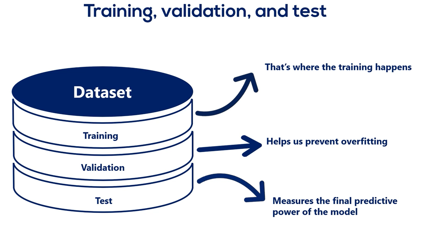
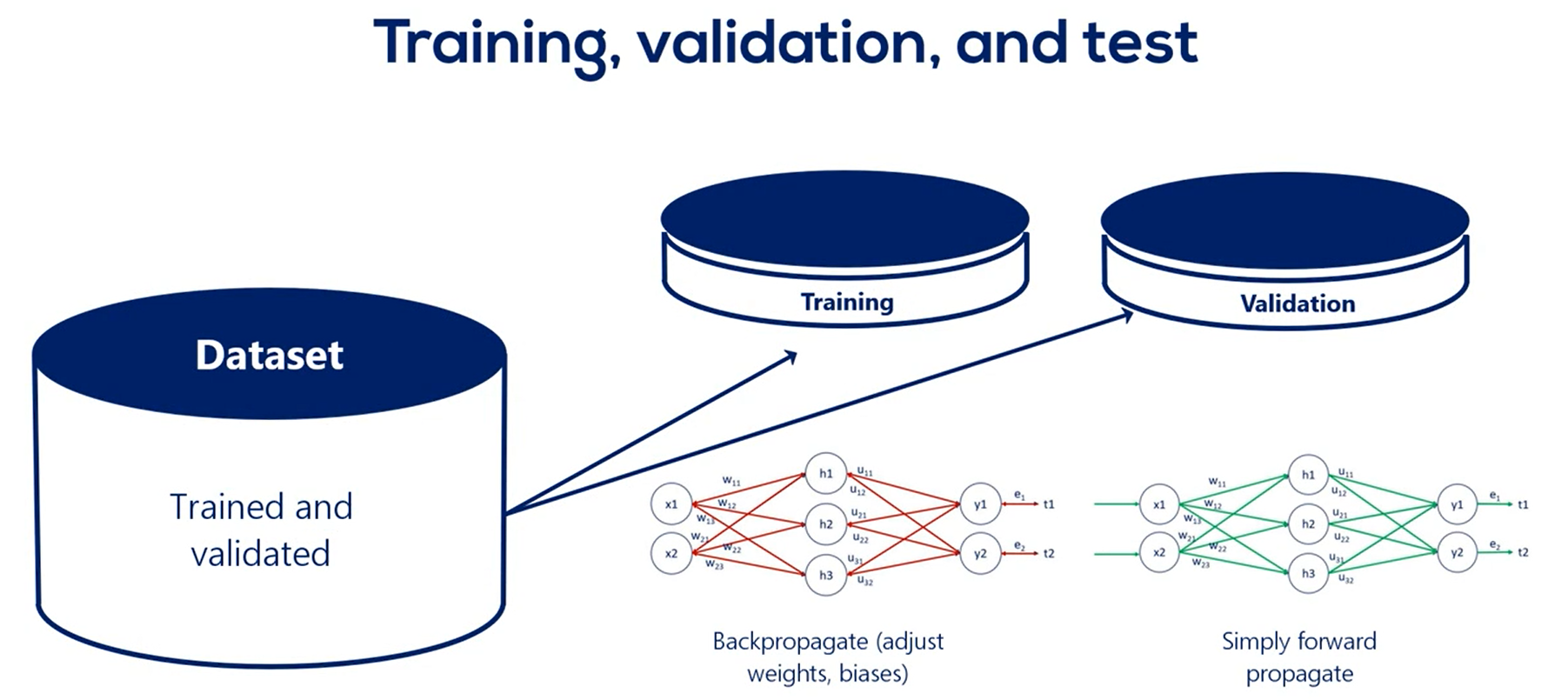
The accuracy of the prediction we get from this test is the accuracy we would expect the model to have if we deploy in real life, so the test data set is the last step we take.

Let's summarize:

First, You get a data set.

Second, you split it into three parts.

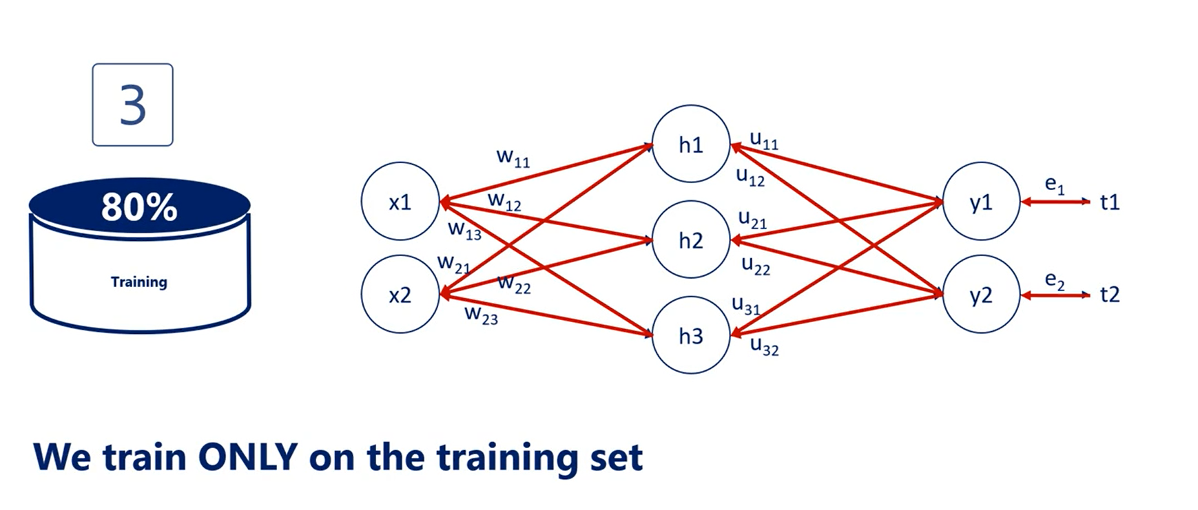
There is no set rule but splits like 80 percent training 10 percent validation and 10 percent test or 70 2010 are commonly used.

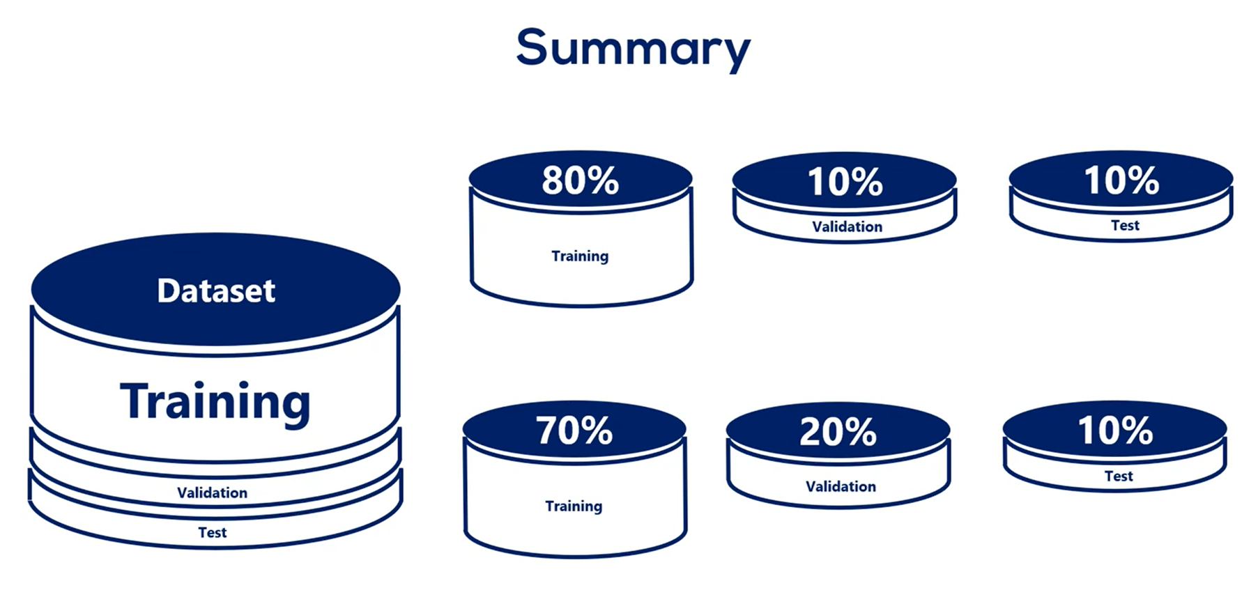
Obviously the data set where we treat the model should be considerably larger than the other two. You want to devote as much data as possible to the training of the model while having enough samples to validate and test on.

Third, we train the model using the training data set and the training data set only.

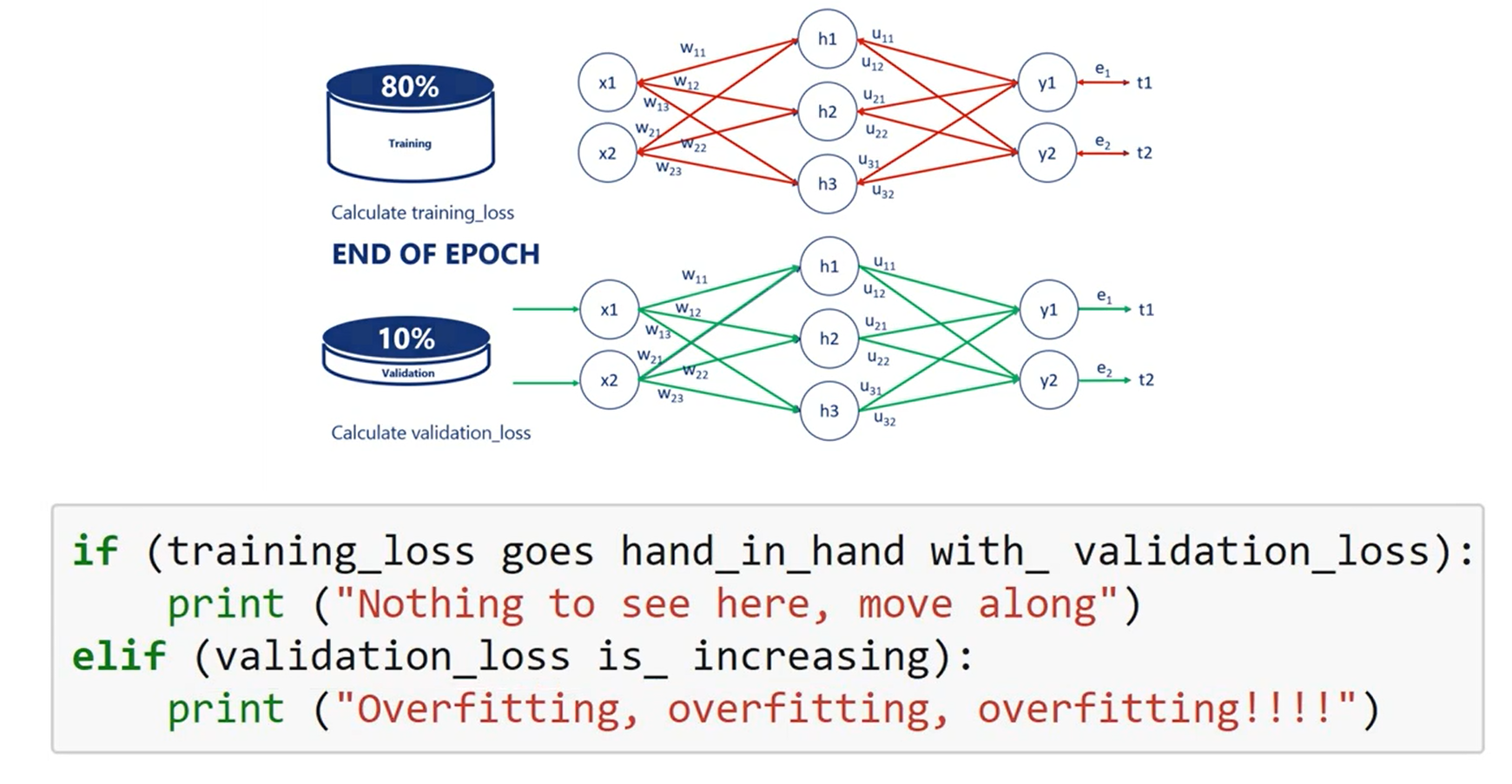
Forth, every now and then we validate the model by running it for the validation data set.

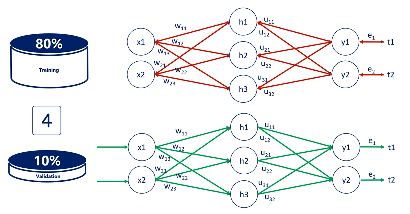
Usually we validate the data set for every epoch, every time we adjust all weights and calculate the training loss, we validate.

if the training loss and the validation loss go hand-in-hand we carry on training the model. If the validation loss is increasing we are overfitting, so we should stop.

Fifth and final step.

You test the model with the test data set the accuracy you obtain at this stage is the accuracy of your machine learning algorithm.

N-fold cross validation

This is a strategy that resembles the general one but combines the train and validation data sets in a clever way. However, it still requires a test subset.

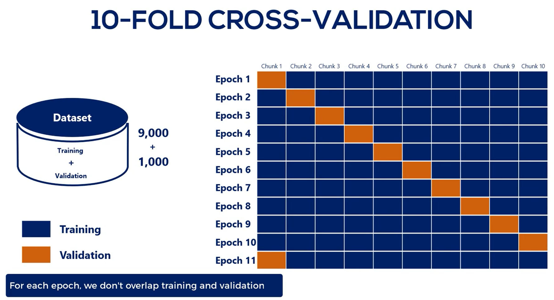
As with all good things this comes at a price we have still trained on the validation set which was not a good idea. It is less likely that the overfitting flag is raised and it is possible that we all were fitted a bit.

The tradeoff is between not having a model or having a model that's a bit over fitted and fold cross-validation solves the scarce data issue but should by no means be used as the norm.

Whenever you can, divide your data into three parts: training, validation and test.

Only if it doesn't manage to learn much because of data scarce it you should try the old cross-validation.

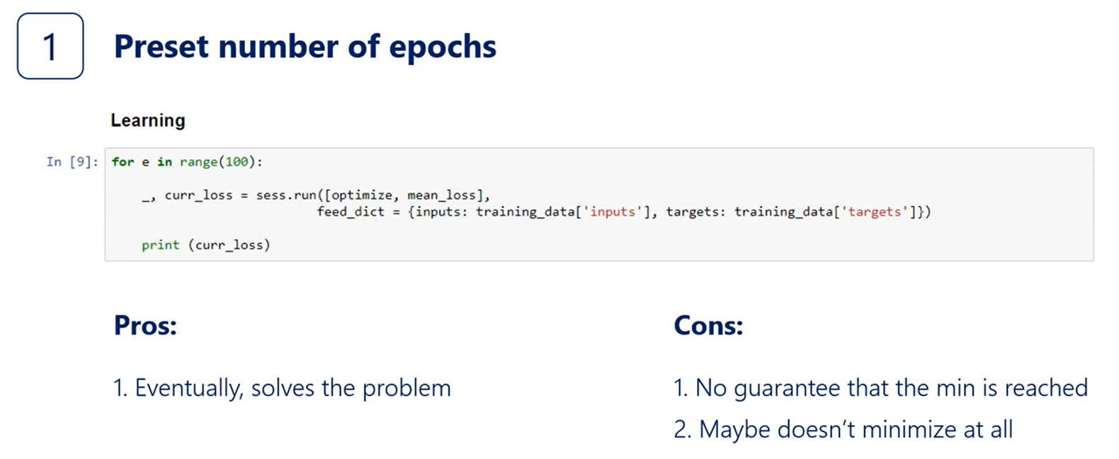
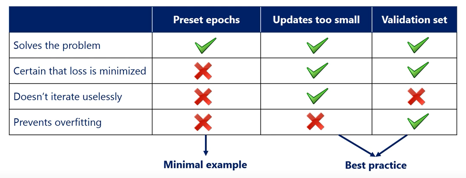
Early stopping

The simplest one is to train for a pre-set number of epochs in the minimal example after the first section.

This gave us no guarantee that the minimum has been reached or passed a high enough learning rate would even cause the loss to divert to infinity.

Still, the problem was so simple that rookie mistakes aside very few epochs would cause a satisfactory result.

However, our machine learning skills have improved so much, and we shouldn't even consider using this naive method.

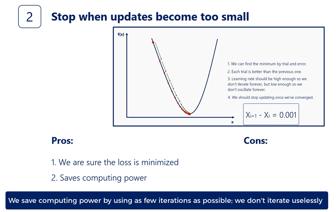
A bit more sophisticated technique is to stop when the last function updates become sufficiently small.

We even had a note on that when we introduce the gradient descent a common rule of thumb is to stop when the relative decrease in the loss function becomes less than 0.001 or 0.1 percent.

This simple rule has two underlying ideas.

First, we are sure we won't stop before we have reached a minimum. That's because of the way gradient descent works. It will descend until a minimum is reached.

The last function will stop changing making the update rule yielding in the same weights. In this way we'll be stuck in the minimum.

The second idea is that we want to save computing power by using as few iterations as possible.

As we said once we have reached the minimum or diverged to infinity we will be stuck there knowing that a gazillion more epochs won't change a thing.

We can just stop there.

This saves us the trouble of iterating uselessly without updating anything.

The third is the best way.

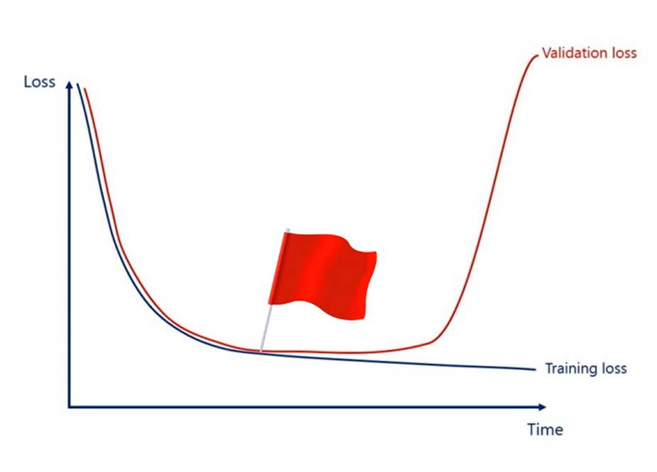
Let me state the rule once again using the proper figure a typical training occurs this way as time goes by the error become smaller.

The distribution is exponential as initially we are finding better weights quickly.

The more we train the model the harder it gets to achieve an improvement. At some point it becomes almost flat.

Now if we put the validation curve on the same graph it would start with the training cost at the point when we started overfitting the validation cost will start increasing.

Here's the point I wish the two functions begin diverging.

That's our red flag. We should stop the algorithm before we do more damage to the model.

Now depending on the case. Different types of early stopping can be used the preset number of iterations method was used in the minimal example.

That wasn't by chance. The problem was linear and super simple. A more complicated method for early stopping would be a stretch.

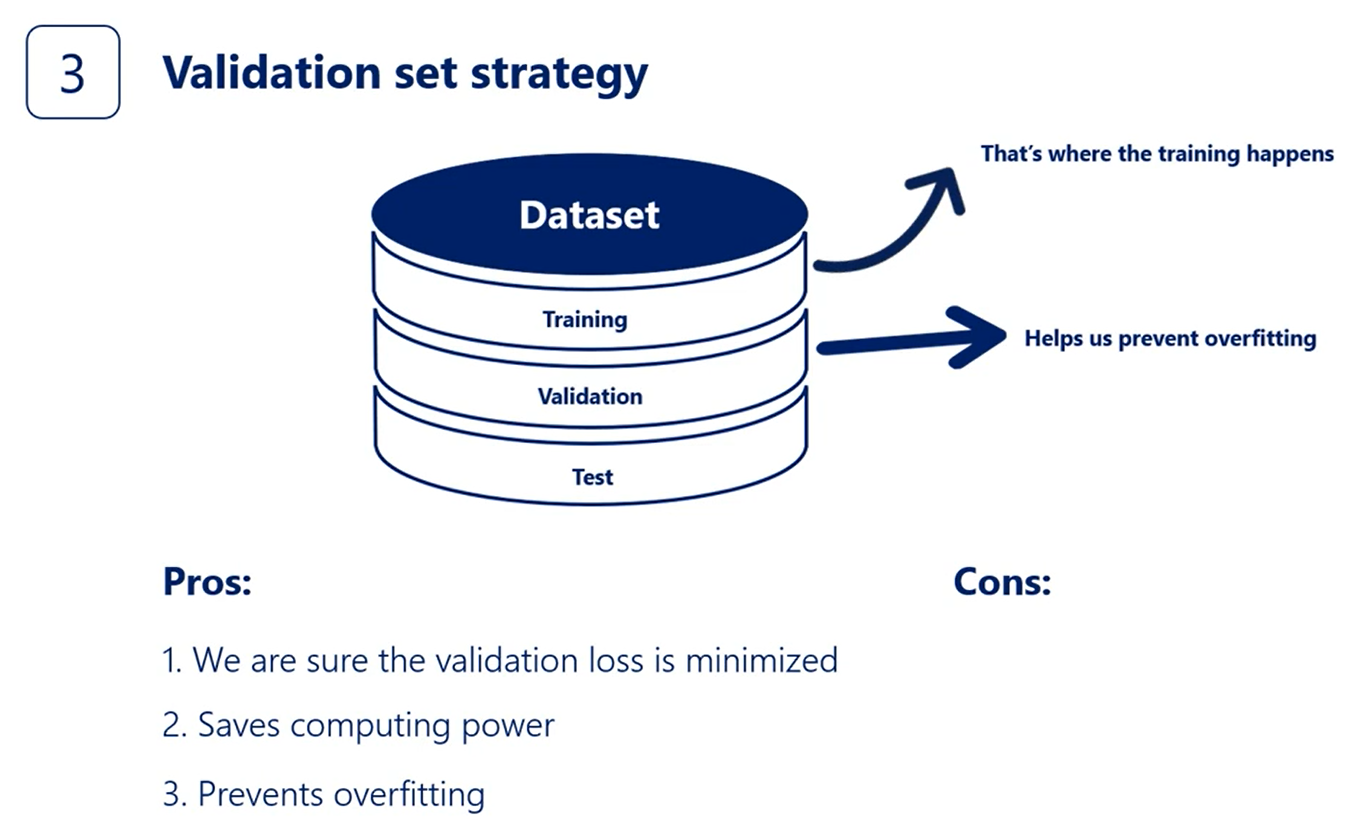
The second method that monitors the relative change is simple and clever but doesn't address overfitting.

The validation set strategy is simple and clever and it prevents overfitting.

However, it may take our algorithm a really long time to overfit it is possible that the weights are barely moving, and we still haven't started overfitting.

That's why I like to use a combination of both methods.

So my rule would be stop when the validation loss starts increasing or when the training last becomes very small.

Initialization

Initialization is the process in which we set the initial values of weights. It was important to add to this section to the Course as an inappropriate initialization would cause in an optimizer role model let's revise what we have seen so far.

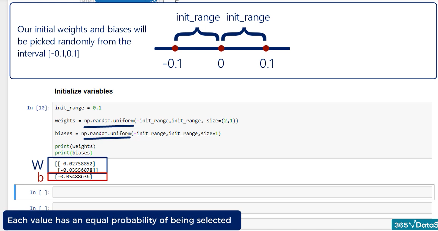
A simple approach would be to initialize weights randomly within a small range.

We did that in the minimal example we use the PI method random uniform and our range was between minus 0.1 and 0.1 this approach chooses the values randomly.

But in a uniform manner each one has the exact same probability of being chosen equal probability of being selected.

Sounds intuitive, but it is important to stress it.

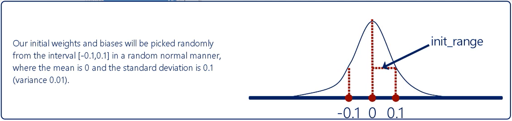
This time though we pick the numbers from a zero mean normal distribution. The chosen variance is arbitrary but should be small.

As you can guess since it follows the normal distribution values closer to 0 are much more likely to be chosen than other values.

An example of such initialization is to draw from a normal distribution with a mean zero, and a standard deviation 0.1.

Both methods are somewhat problematic although they were the norm until 2010. It was just recently that academics came up with a solution.

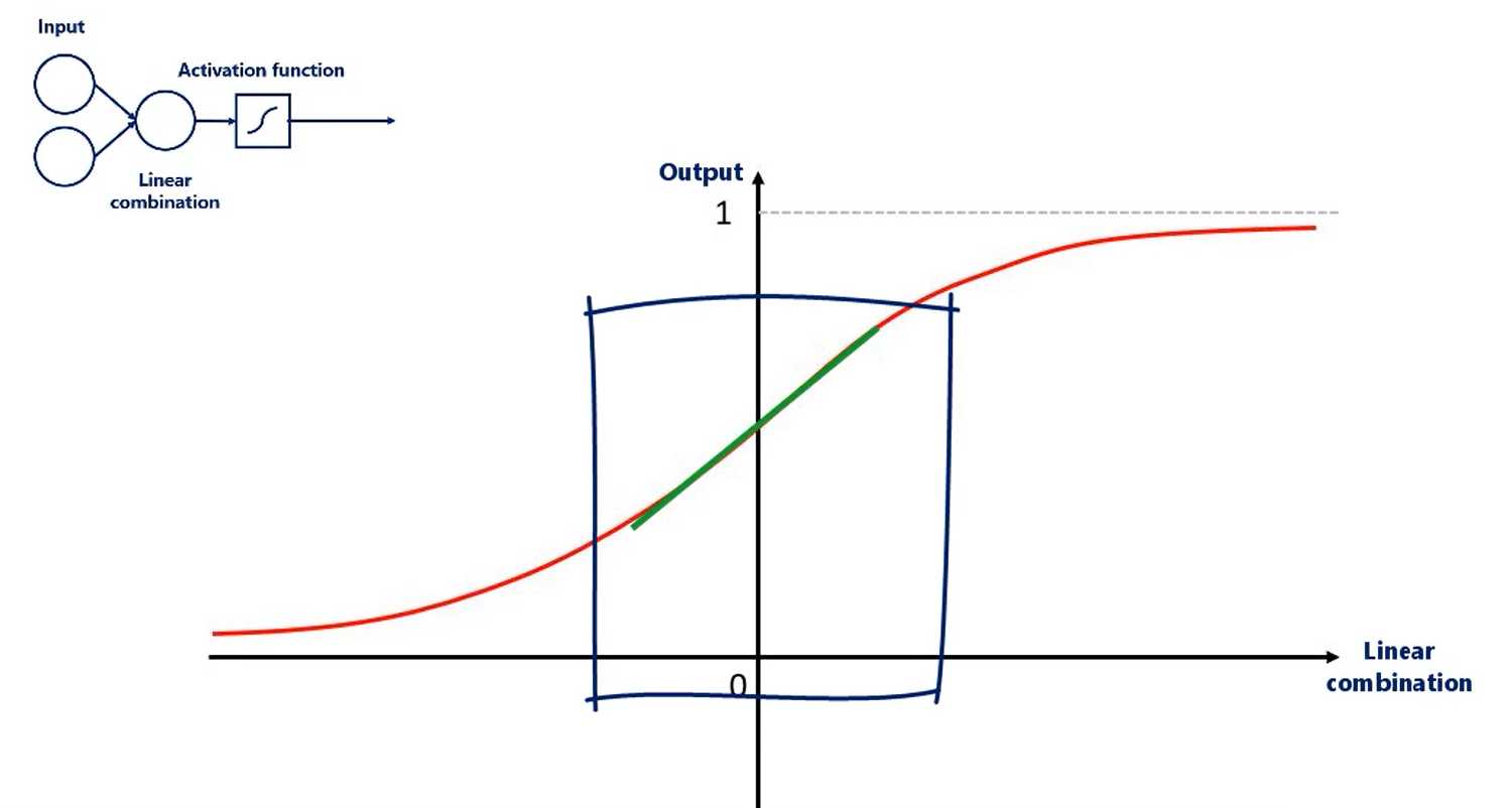
Let's explore the problem. Weights are used in linear combinations then the linear combinations are activated once more we will use the sigmoid activator the sigmoid as other commonly used non-linearities is peculiar around its mean and its Extreme's activation functions take as inputs the linear combination of the units from the previous layer right.

Well if the weights are too small this will cause values that fall around this range in this range.

Unfortunately the sigmoid is almost linear.

If all our inputs are in this range which will happen if we use small weights the sigmoid would not apply nonlinearity but a linearity to the linear combination, and non-linearities are essential for deep nets.

Conversely, if the values are too large or too small the sigmoid is almost flat.

Which cause is the output of the sigmoid to be only once or only zeros respectively a static output of the activations minimises the gradient.

Well, the algorithm is not really trained.

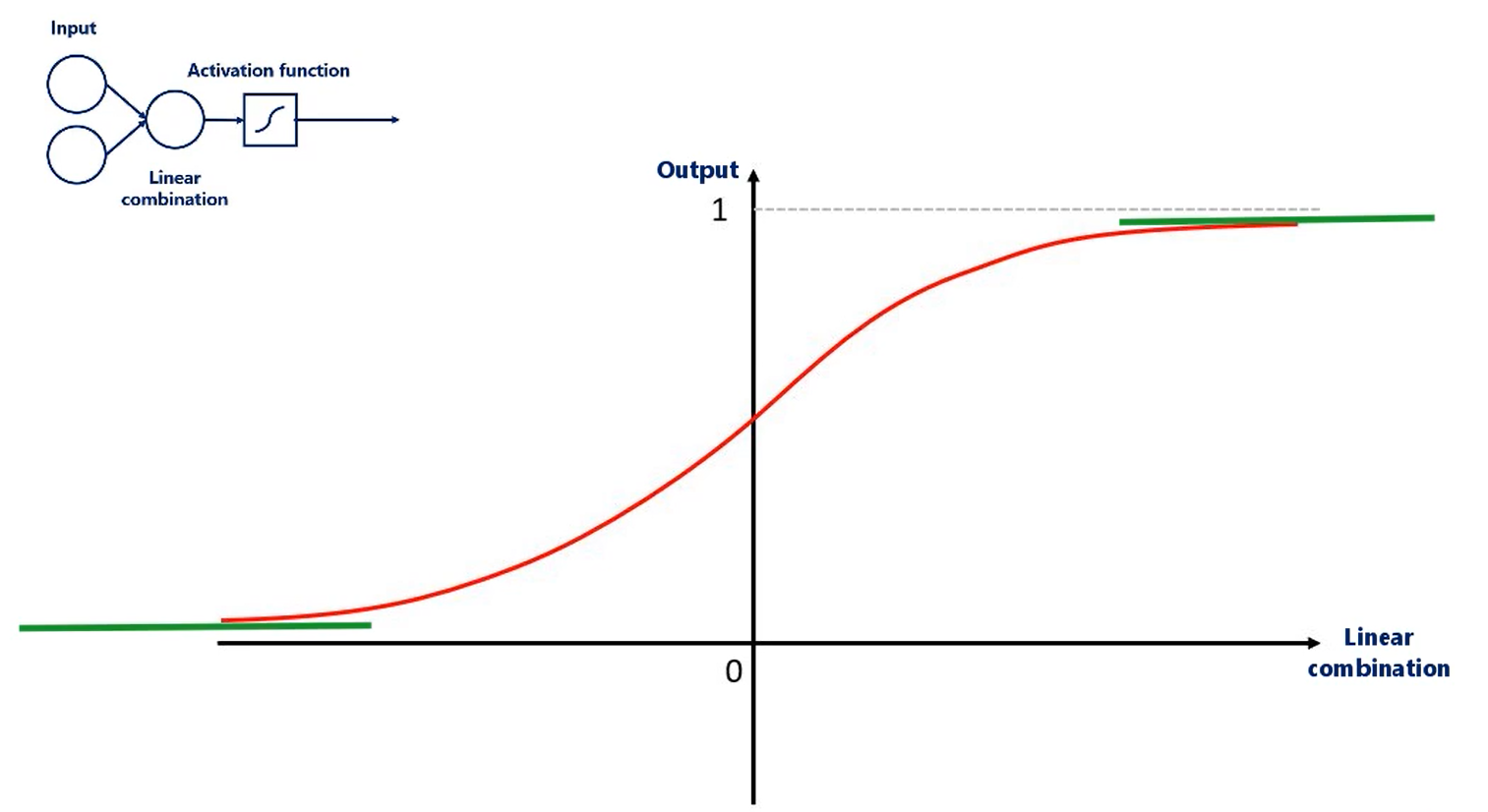
So what we want is a wide range of inputs for this sigmoid. These inputs depend on the weights so the weights will have to be initialized in a reasonable range so we have a nice variance along the linear combinations in the next lesson.

Xavier Initialization

There are both a uniform Xavier initialization and a normal Xavier initialization.

The main idea is that the method used for randomization isn't so important is the number of outputs in the following where that does with the passing of each layer.

The Zeev your initialization is maintaining the variance in some bounds. So we can take full advantage of activation functions. There are two formulas.

The uniform is your initialization States.

We should draw each weight W from a random uniform distribution in the range from minus x to x where x is equal to the square root of 6 divided by the number of inputs plus the number of outputs for the transformation.

For the normal exeat your initialization we have draw each weight W from a normal distribution with a mean of zero and a standard deviation equal to two divided by the number of inputs plus the number of outputs for the transformation the numerator values 2 and 6 vary across sources. But the idea is the same.

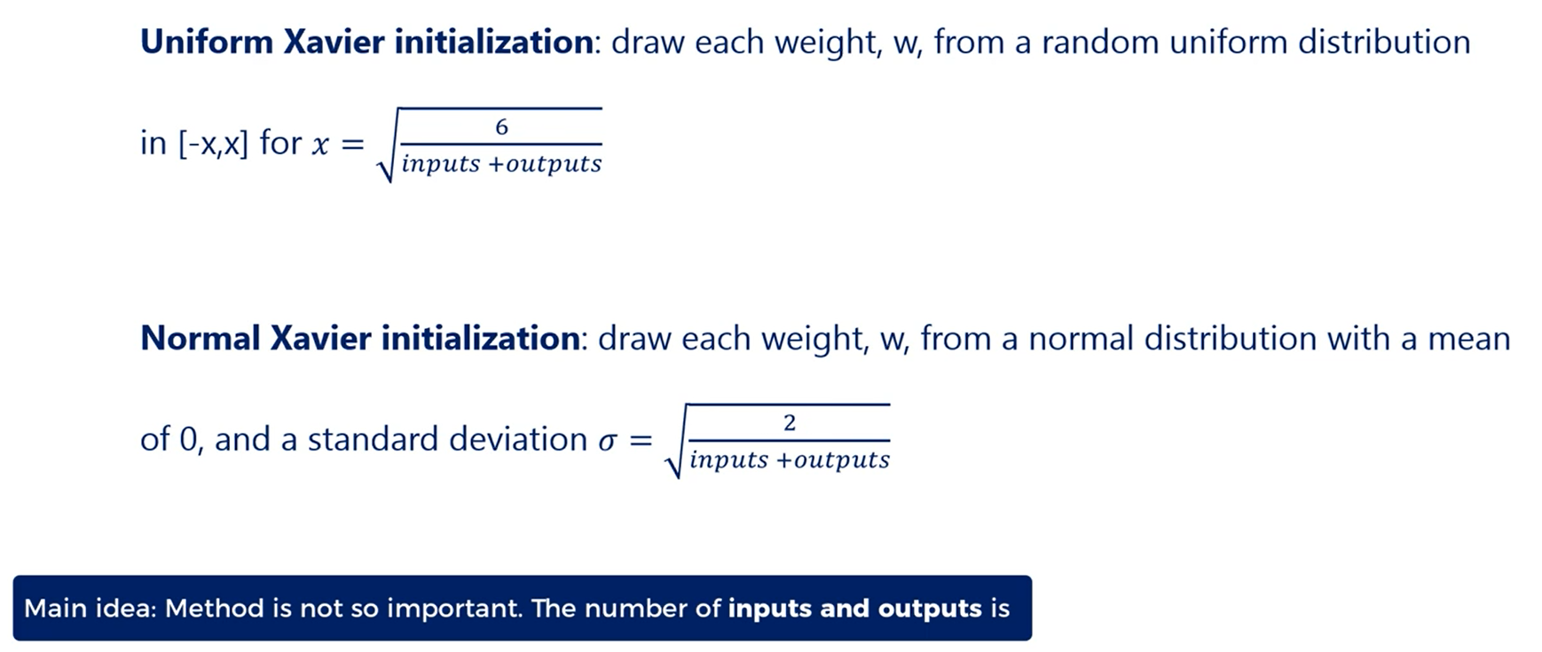
Another detail you should notice is that the number of inputs and outputs matters outputs are clear. That's where the activation function is going.

So the higher number of outputs the higher need to spread weights.

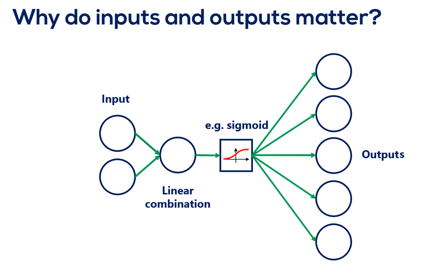
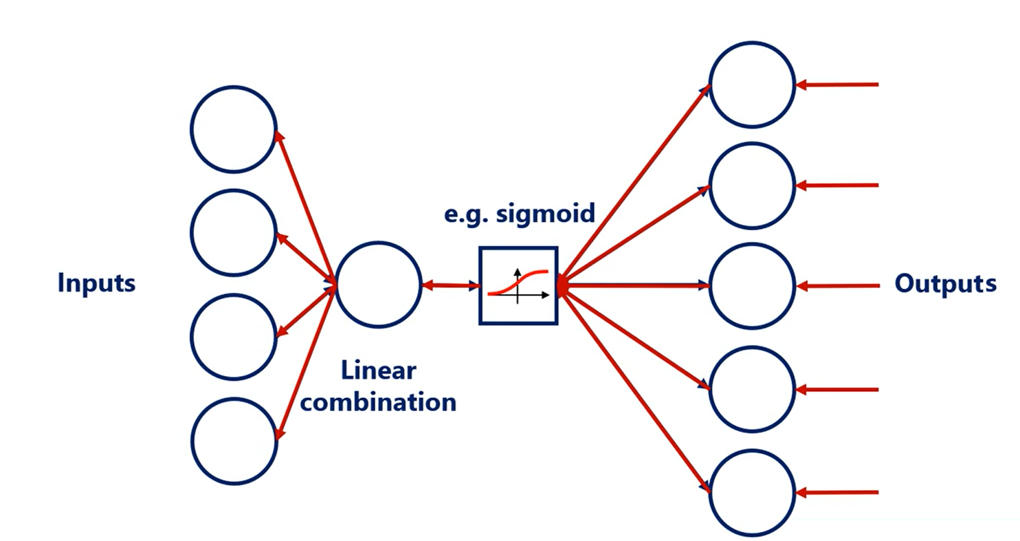
What about inputs?

Well optimization is done through back propagation. So when we back propagate we would obviously have the same problem but in the opposite direction.

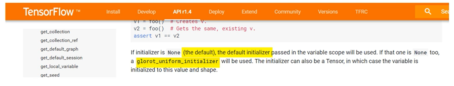
Finally, in TensorFlow this is the default initializer.

So if you initialize the variables without specifying how it will automatically adopt the exit of your initializer unlike what we did in the minimal example.

Gradient descent and learning rates

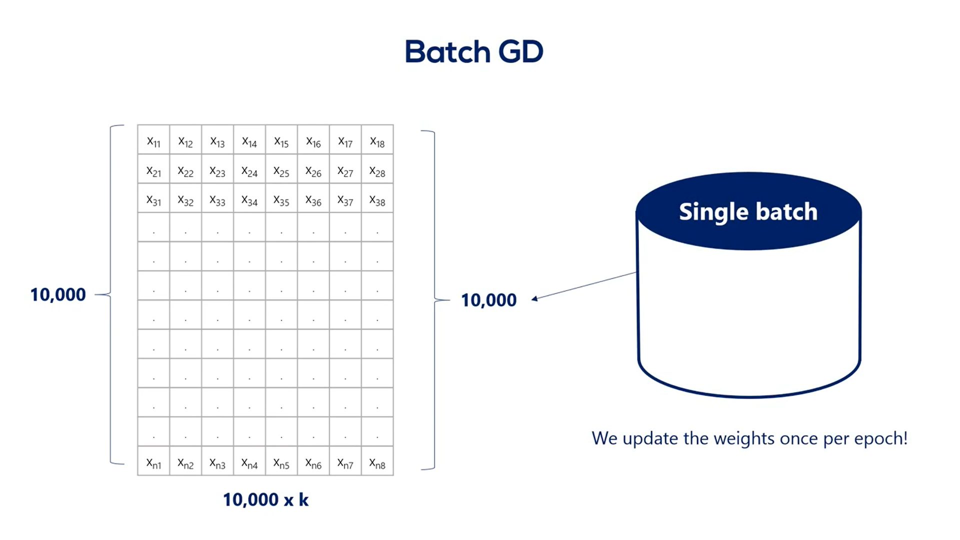
The gradient descent, GD, short for gradient descent, iterates over the whole training set before updating the weights.

Each update is very small.

That's due to the whole concept of the gradient descent, driven by the small value of the learning rate.

As you remember, we couldn't use a value too high, as this jeopardises the algorithm. Therefore, we have many epochs over many points using a very small learning rate.

This is slow.

It's not descending.

It's basically snailing down the gradient.

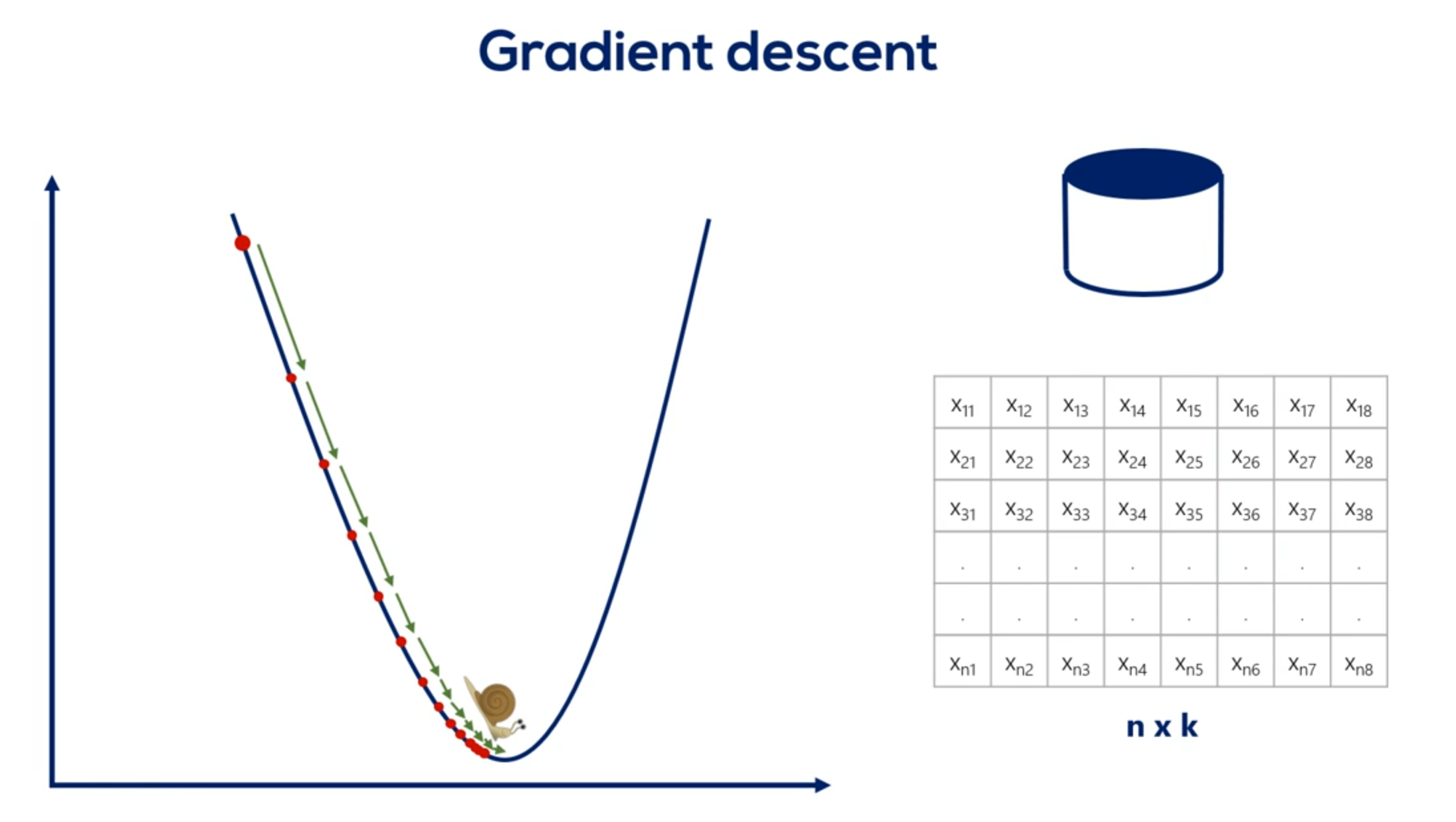
Fortunately for us, there is a simple solution to the problem.

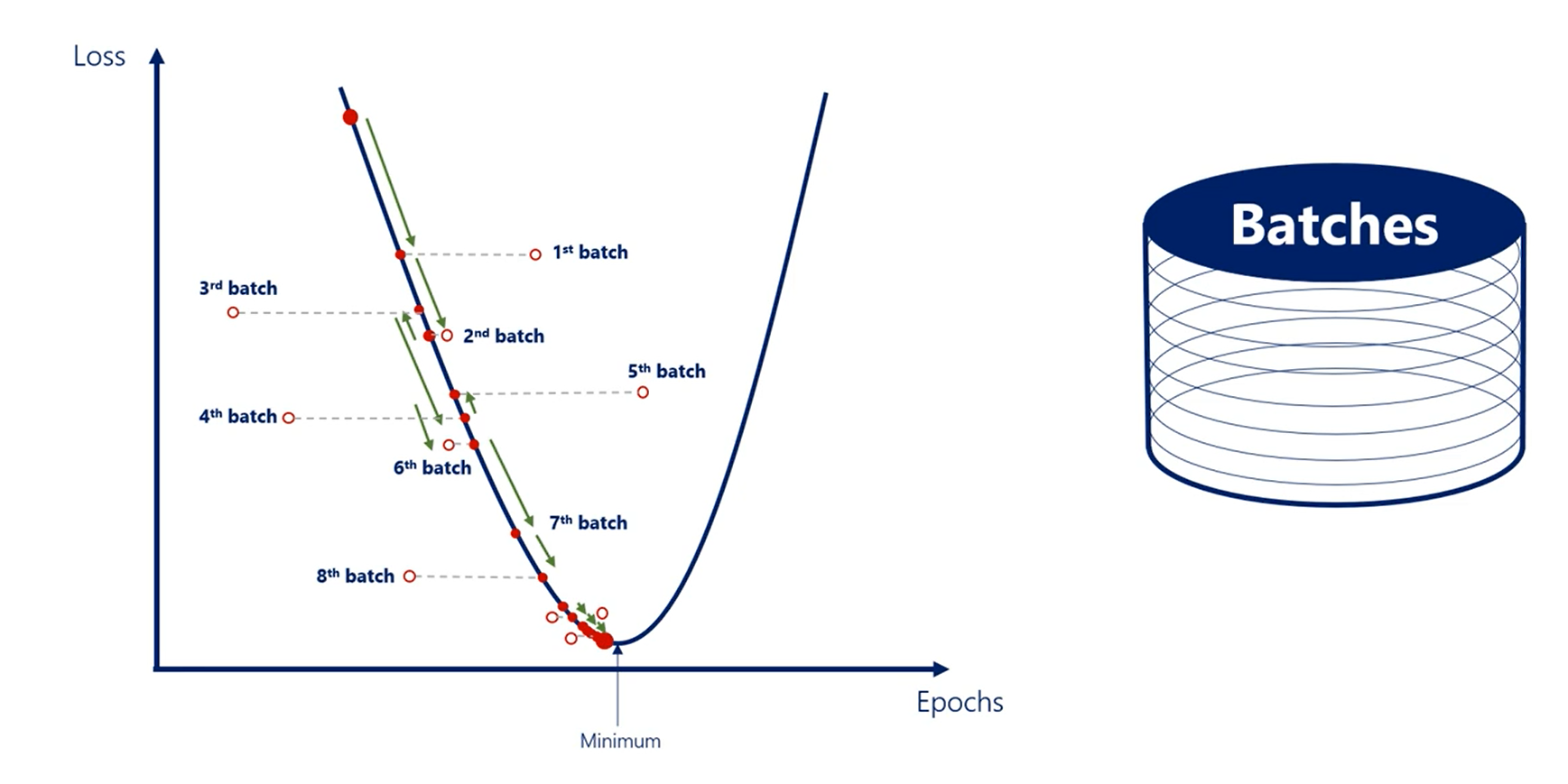
It's a similar algorithm called the SGD or the stochastic gradient descent.

It works in the exact same way, but instead of updating the weights once per epoch it updates them in real time inside a single epoch.

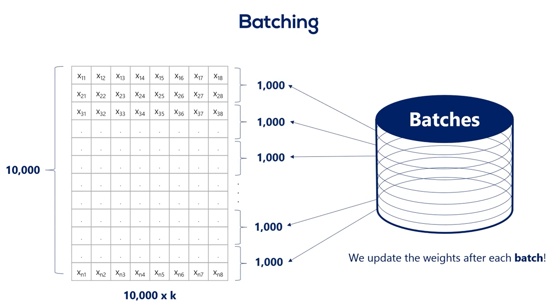
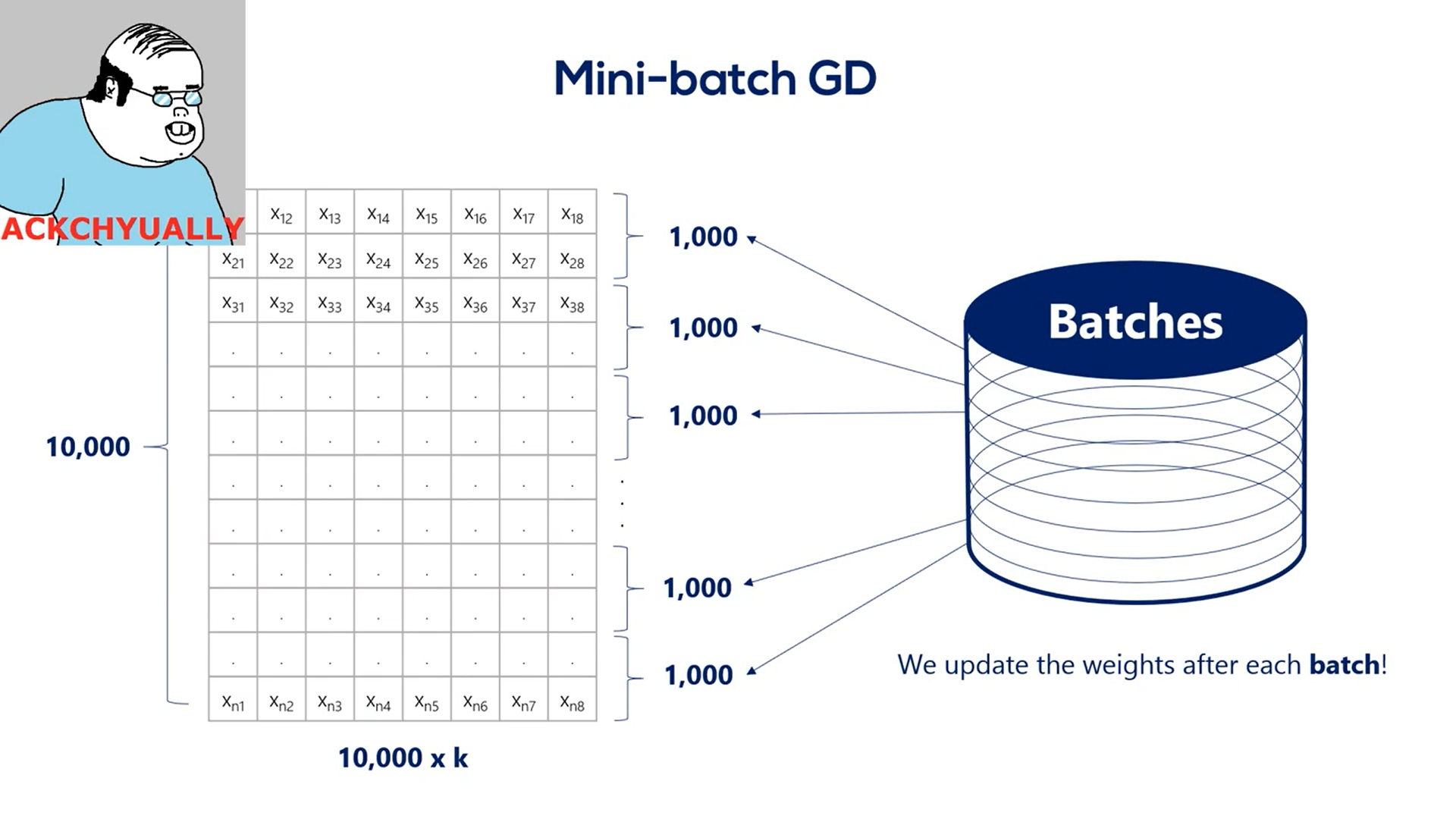
The stochastic gradient descent is closely related to the concept of batching.

Batching is the process of splitting data into and batches often called many batches.

We update the weights after every batch instead of every epoch.

Let's say we have 10000 training points. If we choose a batch size of 1000 then we have 10 batches per epoch. So for every full iteration over the training data set we would update the weights 10 times instead of one.

This is by no means a new method. It is the same as the gradient descent but much faster.

The SGD comes at a cost.

It approximates things a bit.

So, we lose a bit of accuracy, but the tradeoff is worth it.

That is confirmed by the fact that virtually everyone in the industry uses stochastic gradient descent not gradient descent.

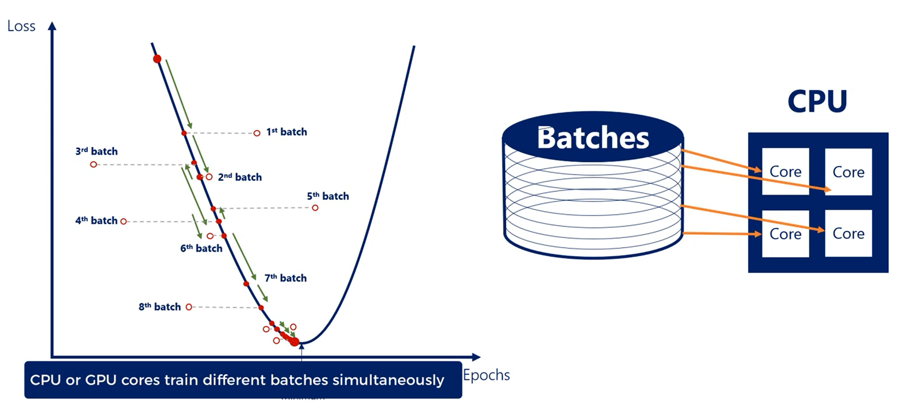
So why does this speed up the algorithm so drastically?

There are a couple of reasons, but one of the finest is related to hardware. Splitting the training set into batches allows the CPU cores or the GPU cores to train on different batches in parallel. This gives an incredible speed boost, which is why practitioners rely on it.

Actually, stochastic gradient descent is when you update after every input. So your batch size is one.

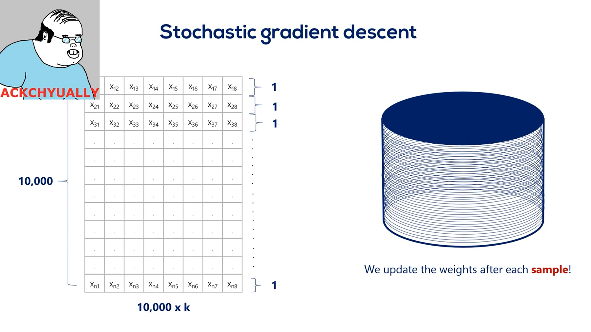
What we have been talking about was technically called mini batch.

Gradient descent However, more often than not, practitioners refer to the mini batch GD as stochastic gradient descent.

If you are wondering, the plane gradient descent we talked about at the beginning of the Course is called batched GD as it has a single batch.

Gradient descent pitfalls

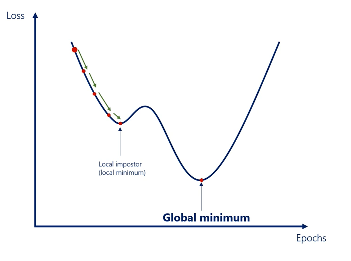
In real life though loss functions are not so regular. What if I told you this was not the whole graph of the last function. It was just one of its minima.

A local imposter rather than the sought extremum zooming out.

We see that actually the global minimum of the loss is this point.

Each local minimum is a suboptimal solution to the machine learning optimization.

Gradient descent is prone to this issue. Often it falls into the closest minimum to the starting point rather than the global minimum.

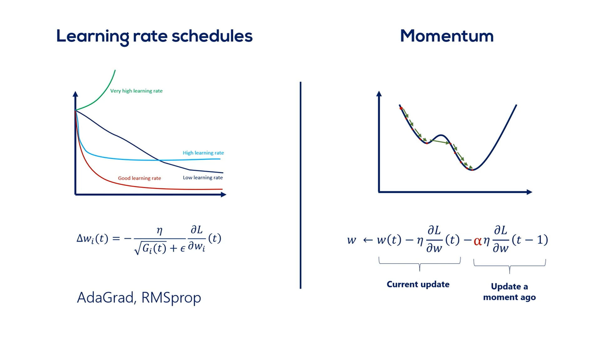
Momentum

The gradient descent and the stochastic gradient descent are good ways to train our models.

We need not change them. We should simply extend them the simplest extension we should apply.

It is called momentum.

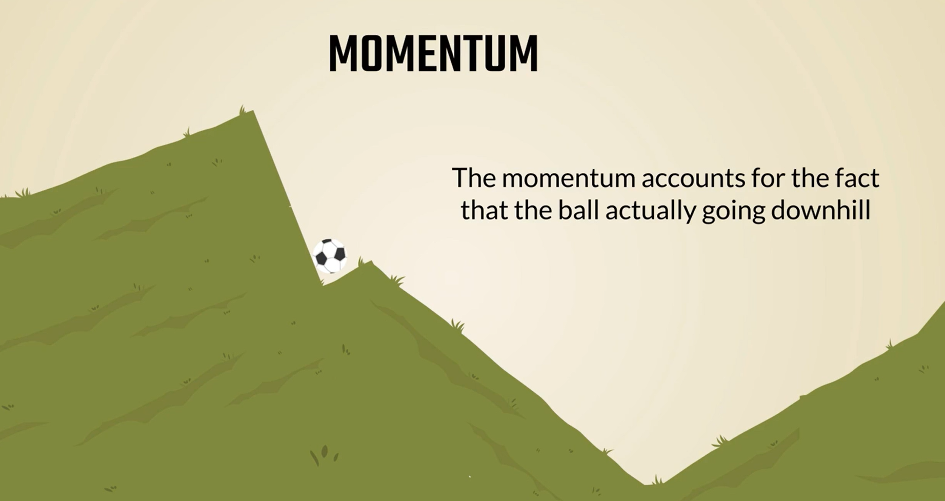
An easy way to explain momentum is through a physics analogy.

Imagine the gradient descent as rolling a ball down a hill. The faster the ball rolls the higher is its momentum.

A small dip in the grass would not stop the ball it would rather continue rolling until it has reached a flat surface out of which it cannot go.

The small dip is the local minimum while the Big Valley is the global minimum.

If there wasn't any momentum the ball would never reach the desired final destination. It would have rolled with some none increasing speed and would have stopped in the dip.

The momentum accounts for the fact that the ball is actually going downhill.

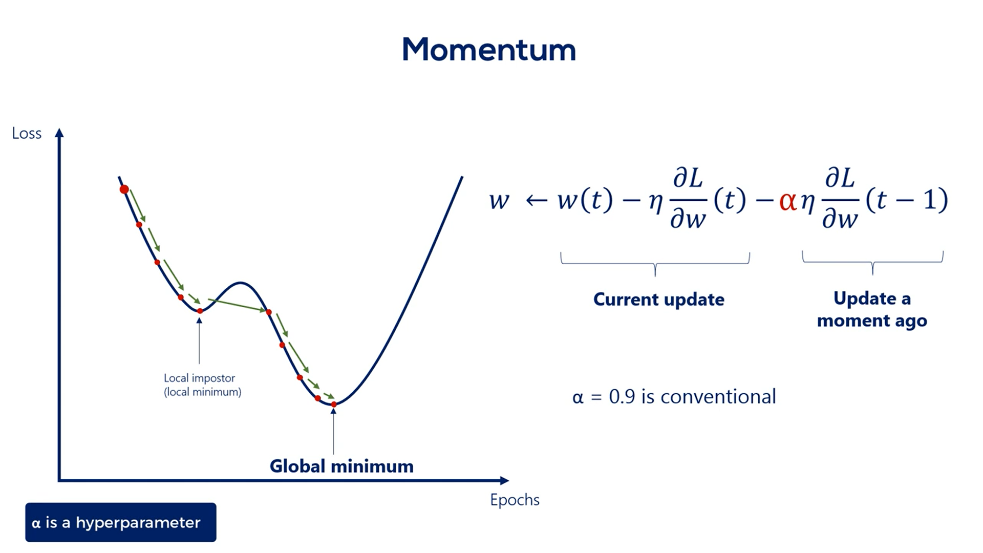
So how do we add momentum to the algorithm?

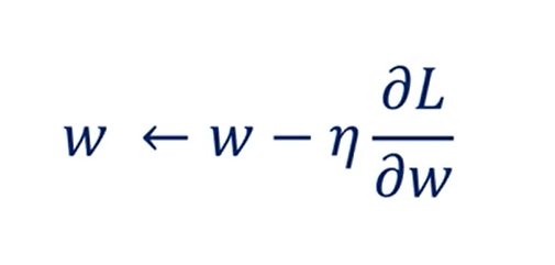
The rule so far was:

Including momentum, we will consider the speed with which we've been descending so far.

For instance, if the ball is rolling fast the momentum is high otherwise the momentum is low.

The best way to find out how fast the ball rolls is to check how fast it rolled a moment ago.

That's also the method adopted in machine learning.

We add the previous update step to the formula. We want to multiplied by some coefficient. Otherwise, we would assign the same importance to the current update and the previous one.

Usually, we use an alpha of 0.9 to adjust the previous update. Alpha is a hyper parameter and we can play around with it for better results.

0.9 is the conventional rule of thumb.

Learning Rates Schedules

Learning rate ( $\eta$ )

$\eta$ must be small enough so we gently descend through the last function instead of oscillating wildly around the minimum and never reaching it, or diverging to infinity.

It also had to be big enough, so the optimization takes place in a reasonable amount of time.

A smart way to deal with choosing the proper learning rate is adopting a so-called learning rate schedule.

There are two basic ways to do that:

The simplest one is setting a pre-determined piecewise constant learning rate.

For example, we can use a learning rate of 0.1 for the first five epochs then 0.01 for the next five and 0.00 one until the end.

This causes the loss function to converge much faster to the minimum and will give us an accurate result.

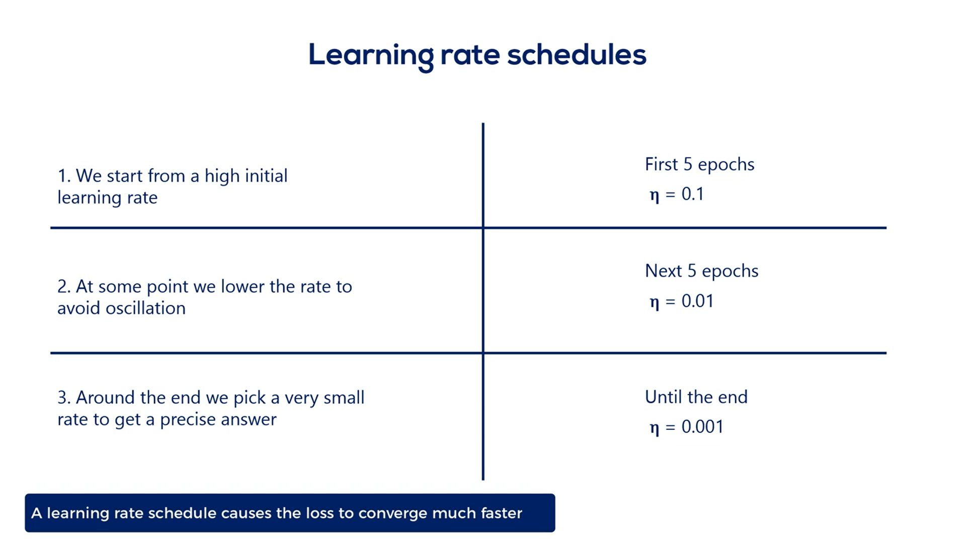
Although, it is crude, as it requires us to know approximately how many Epochs it will take the last to converge. Still, beginners may want to use it as it makes a great difference compared to the constant learning rate.

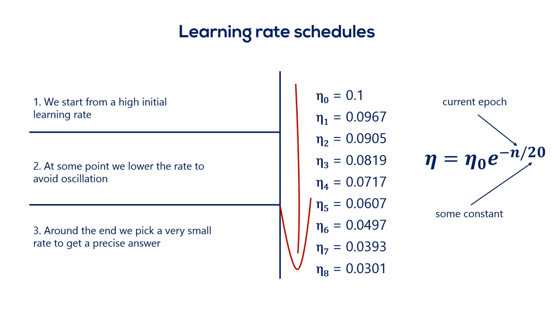
A second much smarter approach is the exponential schedule which is a much better alternative as it smoothly reduces or decays the learning rate.

We usually start from a high value such as $\eta_0 = 0.1$. Then we update the learning rate at each epoch using the rule.

In this expression n is the current epoch while c is a constant. Here's the sequence of learning rates that would follow for a c equal to 20.

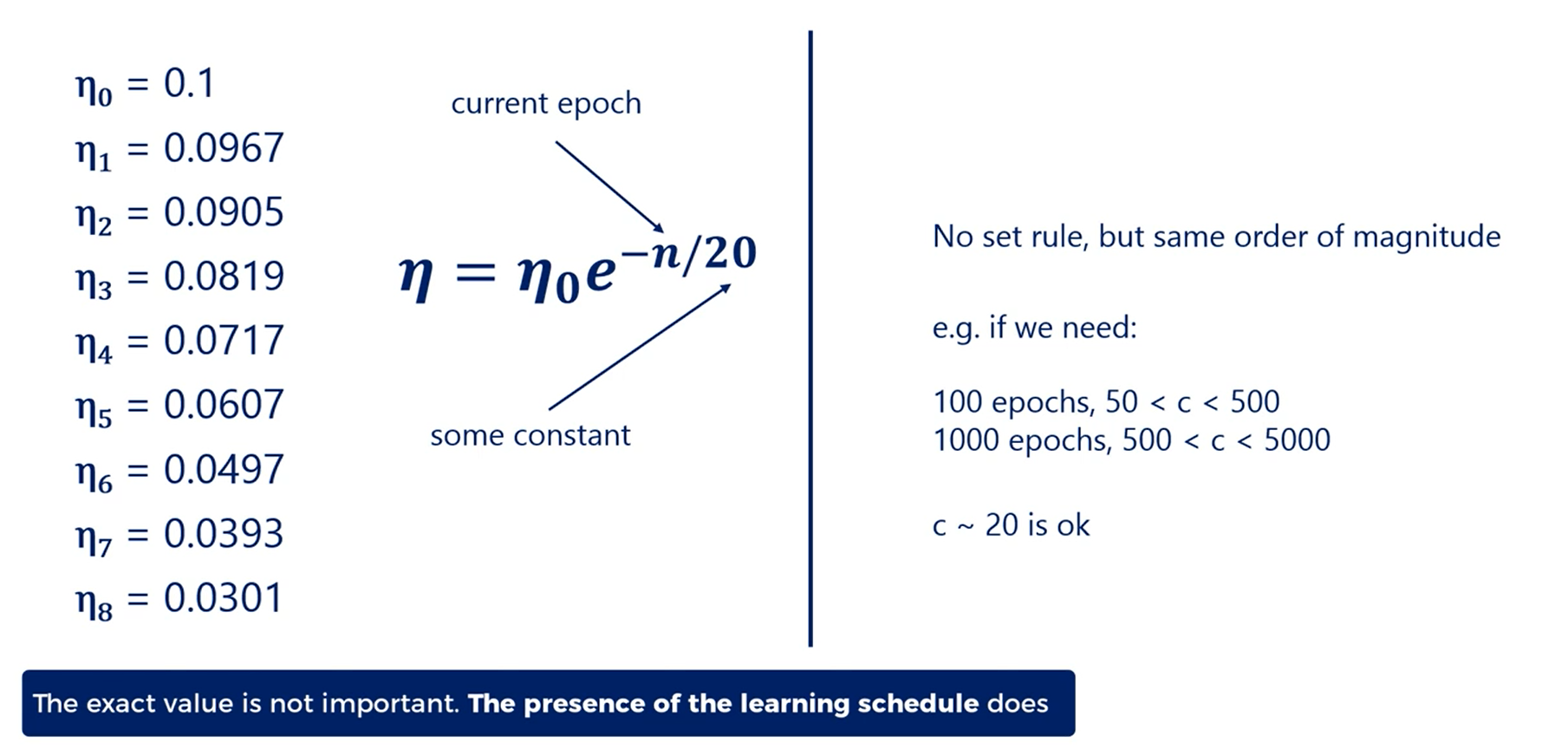
There is no rule for the constant c, but usually it should be the same order of magnitude as the number of epochs needed to minimize the loss.

For example, if we need 100 epochs values of c from 50 to 500 are all fine. If we need 1000 values from 500 to 5000 are alright.

Usually we'll need much less.

So a value of c around 20 or 30 works well.

However,the exact value of c doesn't matter as much. What makes a big difference is the presence of the learning schedule itself.

c is also a hyper parameter.

As with all hyper parameters it may make a difference for your particular problem.

You can try different values of c and see if this affects the results you obtain.

It's worth pointing out that all those cool new improvements such as learning rate schedules and momentum come at a price. We pay the price of increasing the number of hyper parameters for which we must pick values.

Generally, the rule of thumb values work well, but bear in mind that for some specific problem of yours they may not.

It's always worth it to Explore several hyper parameter values before sticking with one

We can see a graph of the loss as a function of the number of epochs.

A well-selected learning rate such as the one defined by the exponential schedule would minimize the loss much faster than a low learning rate.

Moreover, it would do so more accurately than a high learning rate.

Naturally, we are aiming at the good learning rate.

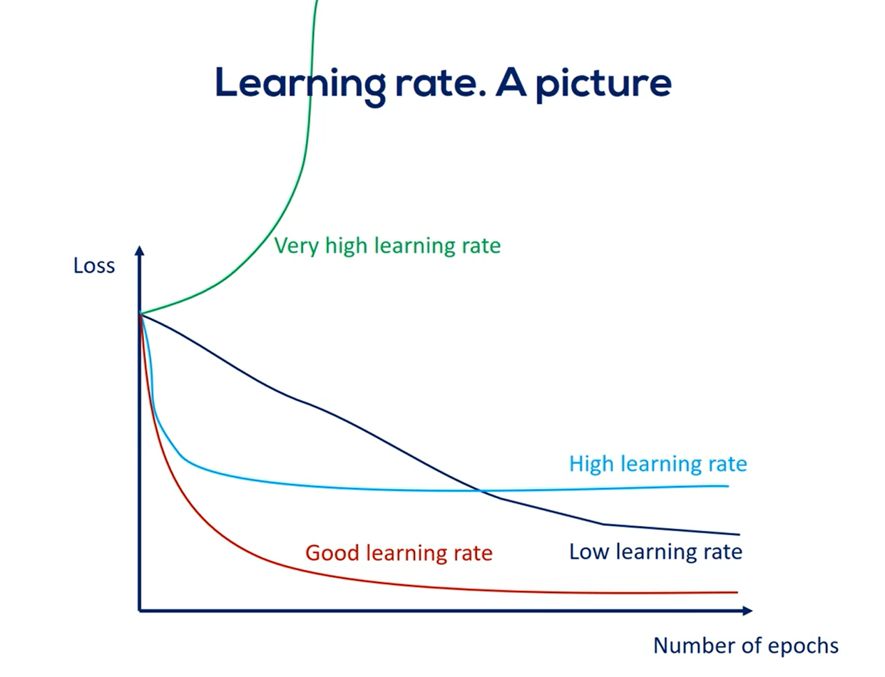
Problem is we don't know what this learning rate is for our particular data model.

One way to establish a good learning rate is to plot the graph we're showing you now for a few learning rate values and pick the one that looks the most like the good curve.

Note that high learning rates may not minimize the loss a low learning rate eventually converges with a good learning rate, but the process will take much longer.

Adaptive learning rate schedules

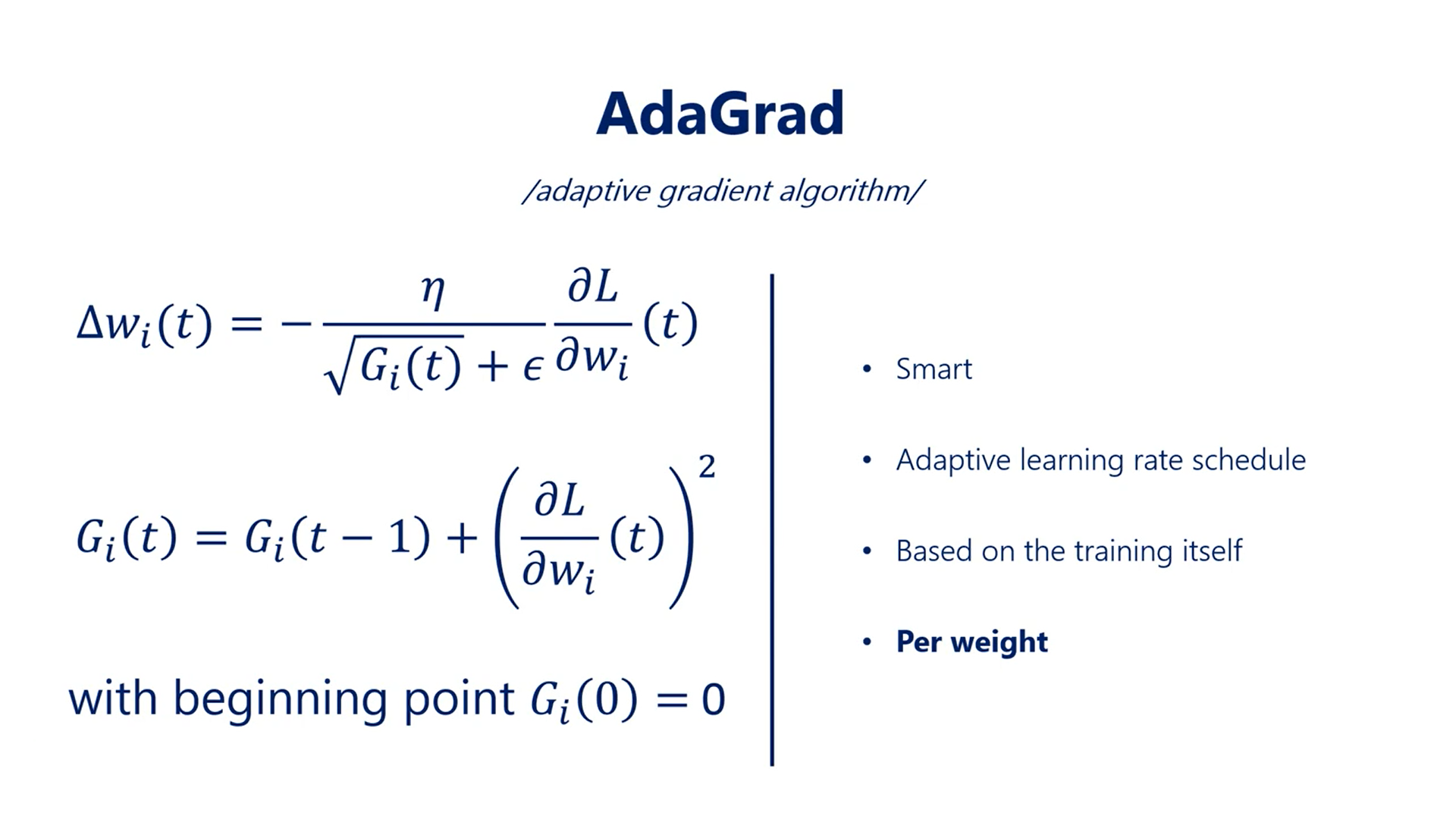
AdaGrad:

It is basically a smart adaptive learning rate scheduler. Adaptive stands for the fact that the effective learning rate is based on the training itself.

It is not a pre-set learning schedule like the exponential one, where all the $\eta$ values are calculated regardless of the training process.

Another very important point is that the adaptation is per weight. This means every individual weight in the whole network keeps track of its own G function to normalize its own steps.

It's an important observation as different weights do not reach their optimal values simultaneously.

The second method is RMSprop or the root mean square propagation.

It is very similar to AdaGrad, the update rule is defined in the same way, but the G function is a bit different.

Empirical evidence shows that in this way the rate adapts much more efficiently.

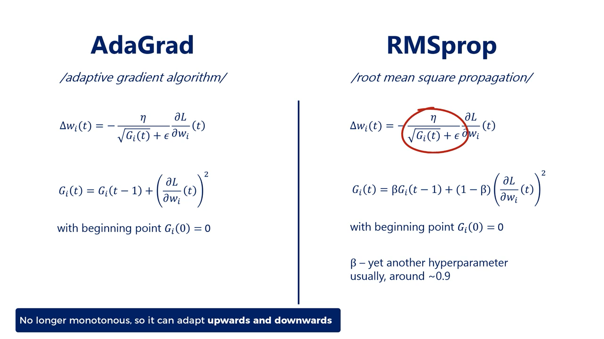
Both methods are very logical and smart.

However, there is a third method based on these two which is superior.

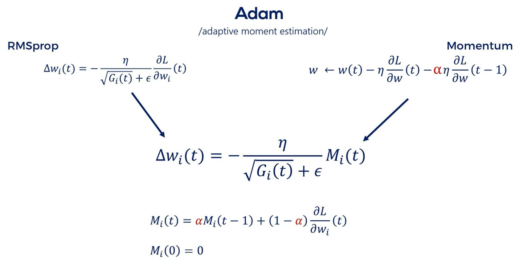
Adaptative Moment Estimation (Adam)

So far we saw two different optimizers each brought a new bright idea to the update rule.

It would be even better if we can combine these concepts and obtain even better results right.

Adam is short for adaptive moment estimation.

If you noticed the AdaGrad and the RMSprop did not include momentum.

Adam steps on RMSprop and introduces momentum into the equation.

TIP

Always use Adam, as it is a cutting edge machine learning method.

Preprocessing

Pre-processing refers to any manipulation we apply to the data set before running it through the model.

Everything we saw so far was conditioned on the fact that we had already preprocessed our data in a way suitable for training.

You've already seen some pre-processing in the TensorFlow intro we created an .npz file all the training we did came from there.

So if you must work with data in an Excel file, csv or whatever saving into an .npz file would be a type of pre-processing.

In this section though we will mainly focus on data transformations rather than reordering as before.

What is the motivation for pre-processing. There are several important points.

• The first one is about compatibility with the libraries we use. As we saw earlier TensorFlow works with tensors and not Excel spreadsheets. In Data Science you will often be given data in whatever format, and you must make it compatible with the tools you use.

• Second we may need to adjust inputs of different magnitude.

• A third reason is generalization.

  Problems that seem different can often be solved by similar models standardizing inputs of different problems allows us to reuse the exact same models.

Basic Preprocessing

We all start with one of the simplest transformations.

Often we are not interested in an absolute value but a relative value that's usually the case when working with stock prices.

If you open Google and type Apple's stock price what you'll get is Apple's stock price but with red or green numbers the relative change in Apple's stock price.

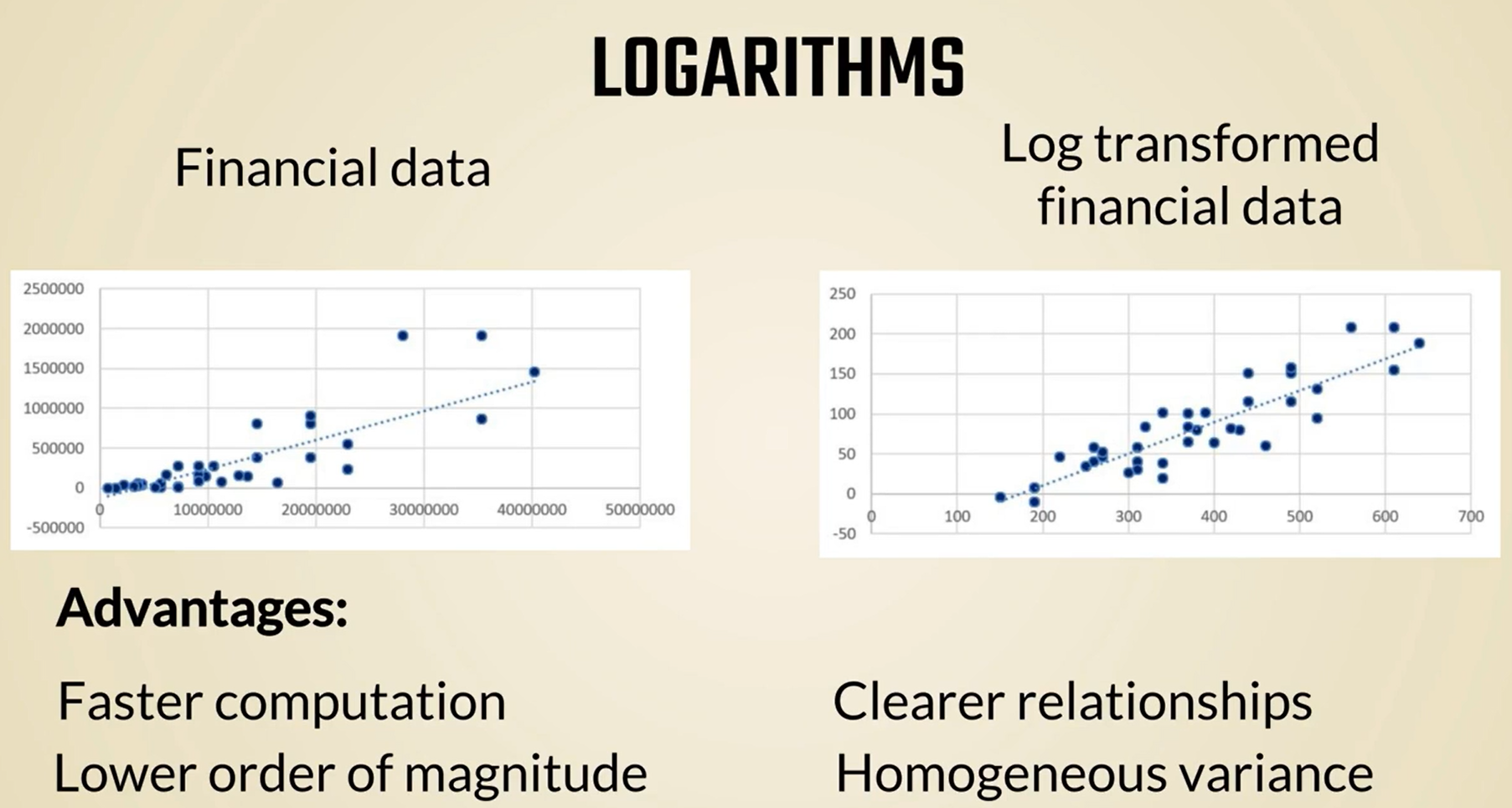
This is an example of pre-processing that is so common we don't consider it as such relative metrics are especially useful when we have a time series data like stock prices Forex exchange rates and so on still in the world of finance we can further transform these relative changes into logarithms many statistical and mathematical methods take advantage of logarithms as they facilitate faster computation in machine learning log transformations are not as common but can increase the speed of learning OK.

So this is one type of pre-processing we wanted to give as an example.

Standardization

The most common problem when working with numerical data is about the difference in magnitudes.

As we mentioned in the first lesson an easy fix for this issue is standardization.

Other names by which you may have heard this term are features scaling and normalization.

However, normalization could refer to a few additional concepts even within machine learning, which is why we will stick with the term standardization and feature scaling.

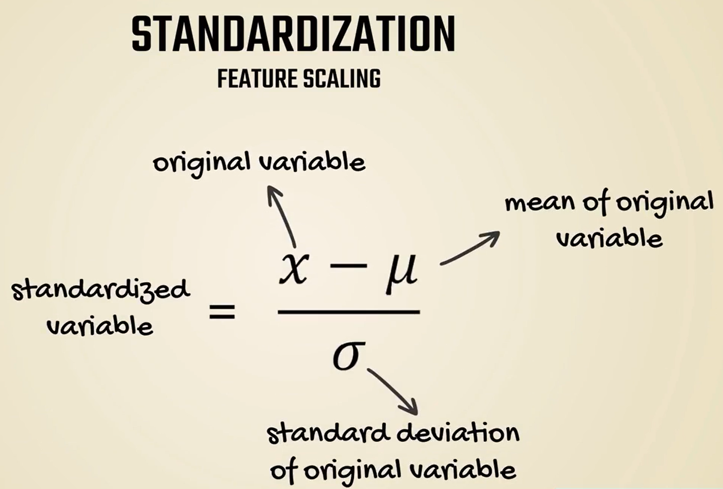
Standardization or feature scaling is the process of transforming the data we are working with into a standard scale.

A very common way to approach this problem is by subtracting the mean and dividing by the standard deviation.

In this way, regardless of the dataset, we will always obtain a distribution with a mean of zero.

Besides standardization, there are other popular methods too.

We will surely introduce them without going too much in detail.

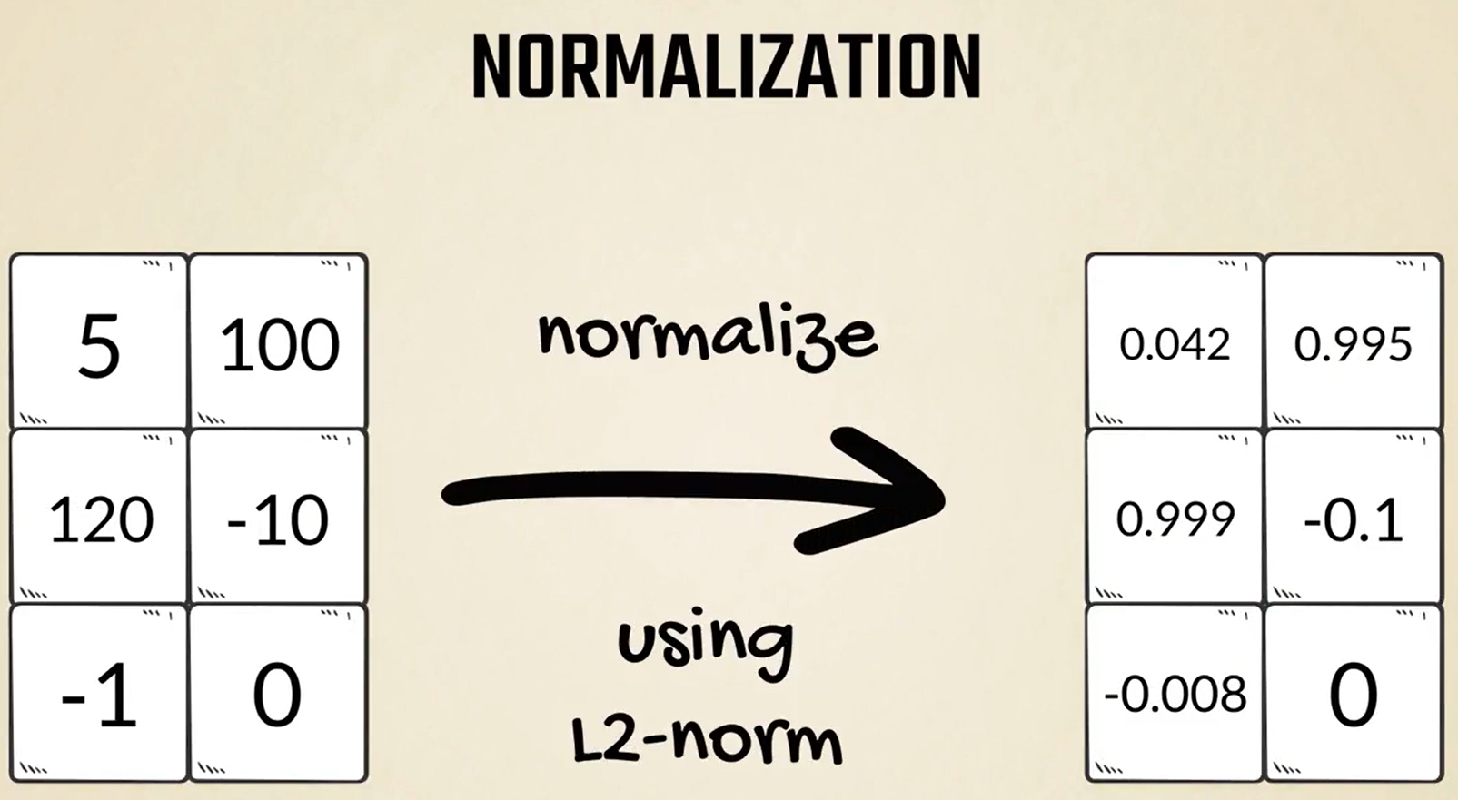
Initially, we said that normalization refers to several concepts.

One of them, which comes up in machine learning, often consists of converting each sample into a unit length vector using the L1 or L2 norm.

Another preprocessing method is PCA standing for principal components analysis.

It is a dimensioned reduction technique, often used when working with several variables referring to the same bigger concept or latent variable.

For instance, if we have data about one's religion voting history participation in different associations and upbringing, we can combine these four to reflect his or her attitude towards immigration.

This new variable will, normally, be standardized in a range with a mean of 0 and a standard deviation of 1.

Whitening is another technique frequently used for pre-processing.

It is often performed after PCA, and removes most of the underlying correlations between data points.

Whitening can be useful when, conceptually, the data should be uncorrelated but that's not reflected in the observations.

We can't cover all the strategies as each strategy is problem specific. However, standardization is the most common one, and is the one we will employ in the practical examples.

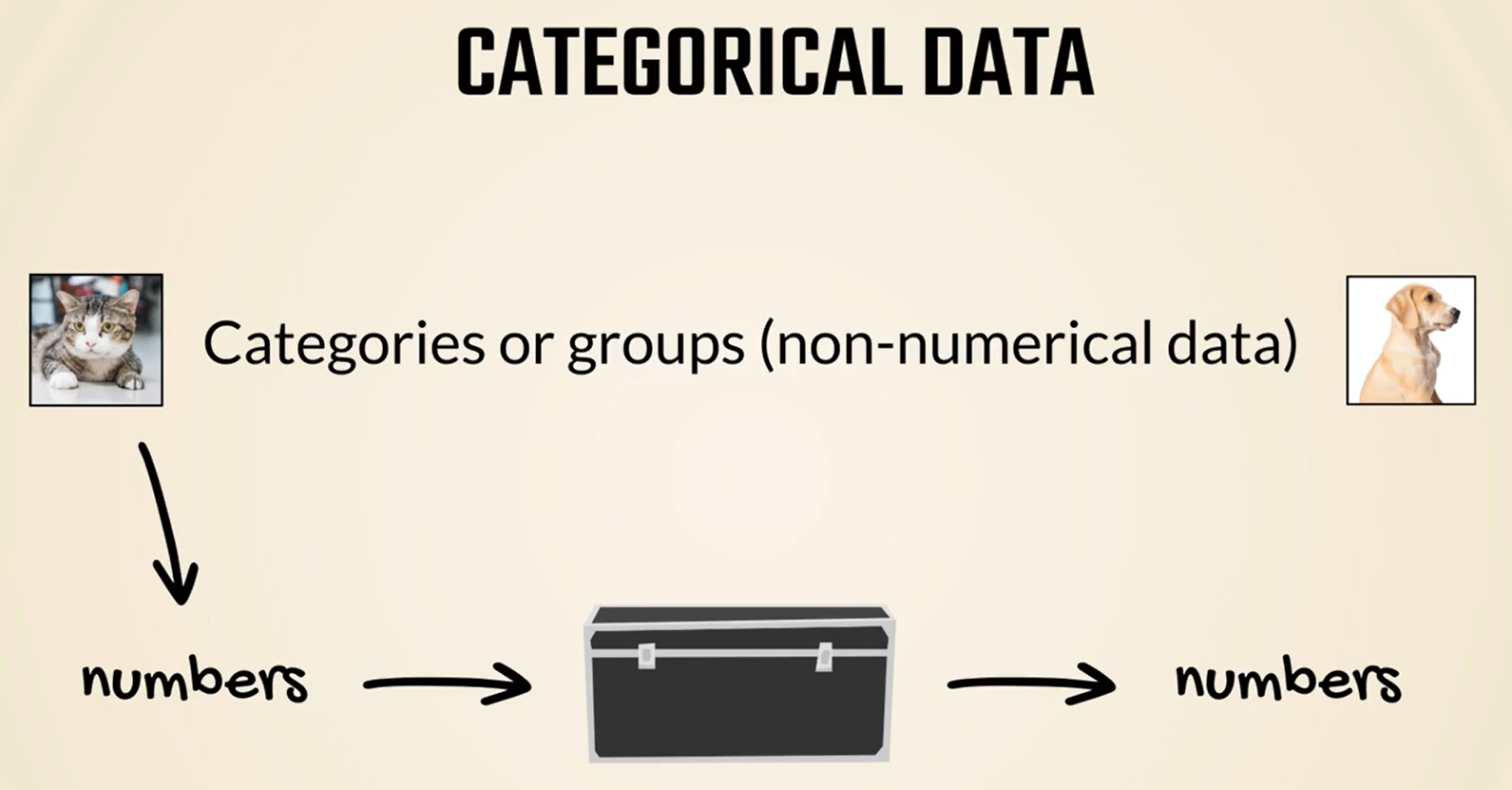
Categorical Data

Often though we must deal with categorical data in short categorical data refers to groups or categories, such as our cat dog examples.

But the machine learning algorithm takes only numbers as values, doesn't it.

Therefore, the question when working with categorical data is: How to convert a cat category into a number, so we can input it into a model or output.

In the end, obviously, a different number should be associated with each category right or better a Tensor.

Binary encoding

Let's introduce binary encoding.

We will start from ordinal numbers.

Bread is represented by the number 1, yogurt by the number 2 and muffin is designated with 3.

Binary encoding implies we should turn these numbers into binary.

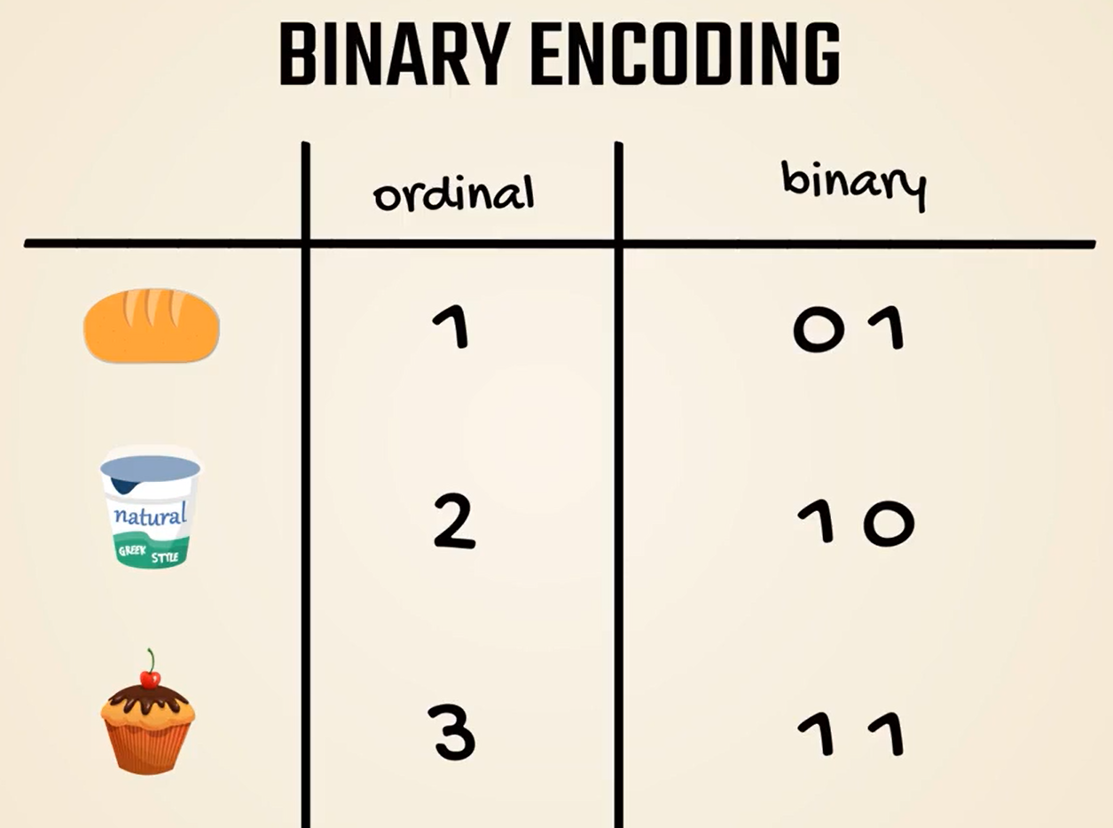
The next step of the process is to divide these into different columns as if we were creating two new variables.

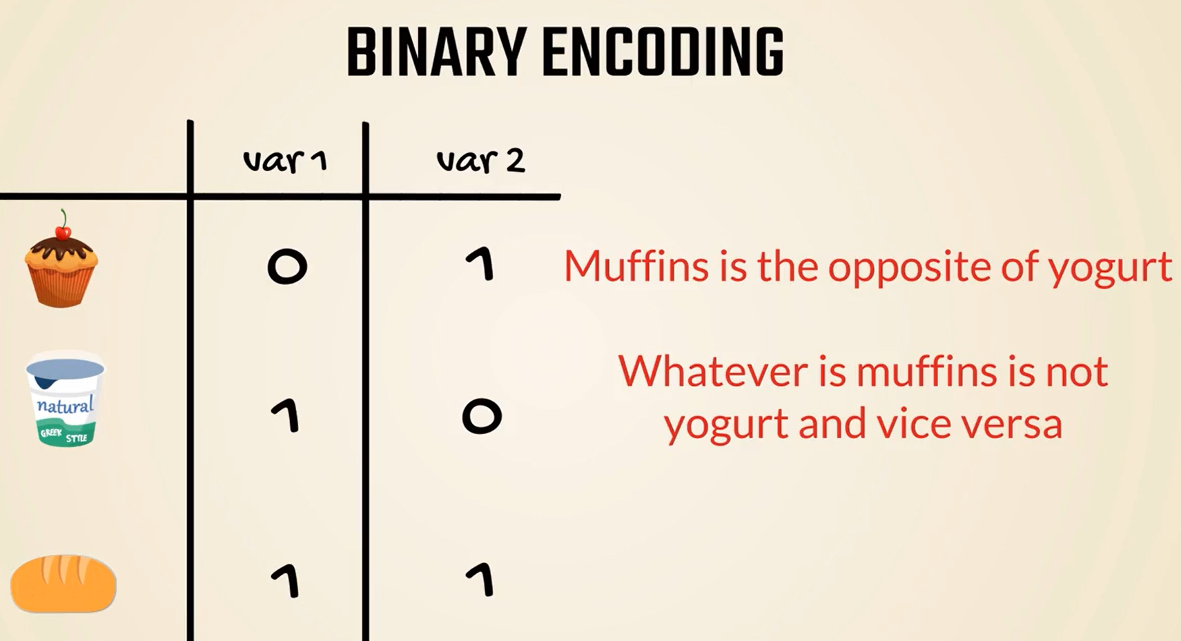
We have differentiated between the three categories and have removed the order.

However, there are still some implied correlations between them.

For instance, bread and yogurt seem exactly the opposite of each other.

Its like we are saying whatever is bread is not yogurt and vice versa.

Even if this makes sense if we encode them in a different way, this opposite correlation would be true for muffins and yogurt but no longer for bread.

Therefore, binary encoding proves problematic, but is a great improvement regarding the initial ordinal method.

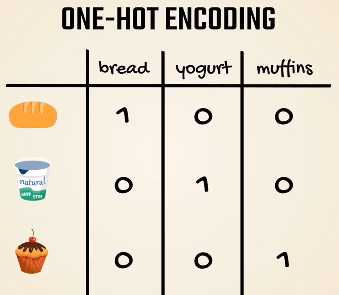
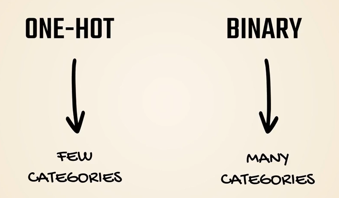
One-Hot encoding

Finally, we have the so called One-Hot encoding one ha is very simple and widely adopted.

It consists of creating as many columns as there are possible values.

Here we have three products thus we need three columns or three variables.

Imagine these variables as asking the question: Is this product bread? Is this product yogurt? and is this product Muffin?

One means yes and Zero means no.

Thus, there will be only one value one and everything else will be zeroed.

This means the products are uncorrelated and unequivocal which is useful and usually works like a charm.

There is one big problem with one high encoding though one encoding requires a lot of new variables.

There is one big problem with one high encoding though one encoding requires a lot of new variables.

For example, Ikea offers around thousand products.

Do we want to include 12000 columns in our inputs.

Definitely not. If we use binary the 12000 products would be represented by 16 columns only since the 12000 product would be written like this in binary.

This is exponentially lower than the 12000 columns we would need for one high encoding.

In such cases we must use binary even though that would introduce some unjustified correlations between the products.

The MNIST problem

How are we going to approach this image recognition problem.

Each image in the amnesty data set is 28 pixels by 28 pixels. It's on a gray scale, so we can think about the problem as a 28 by 28 matrix, where input values are from 0 to 255, 0 corresponds to purely black and 255 to purely white.

For example, a handwritten seven and a matrix would look like this that's an approximation.

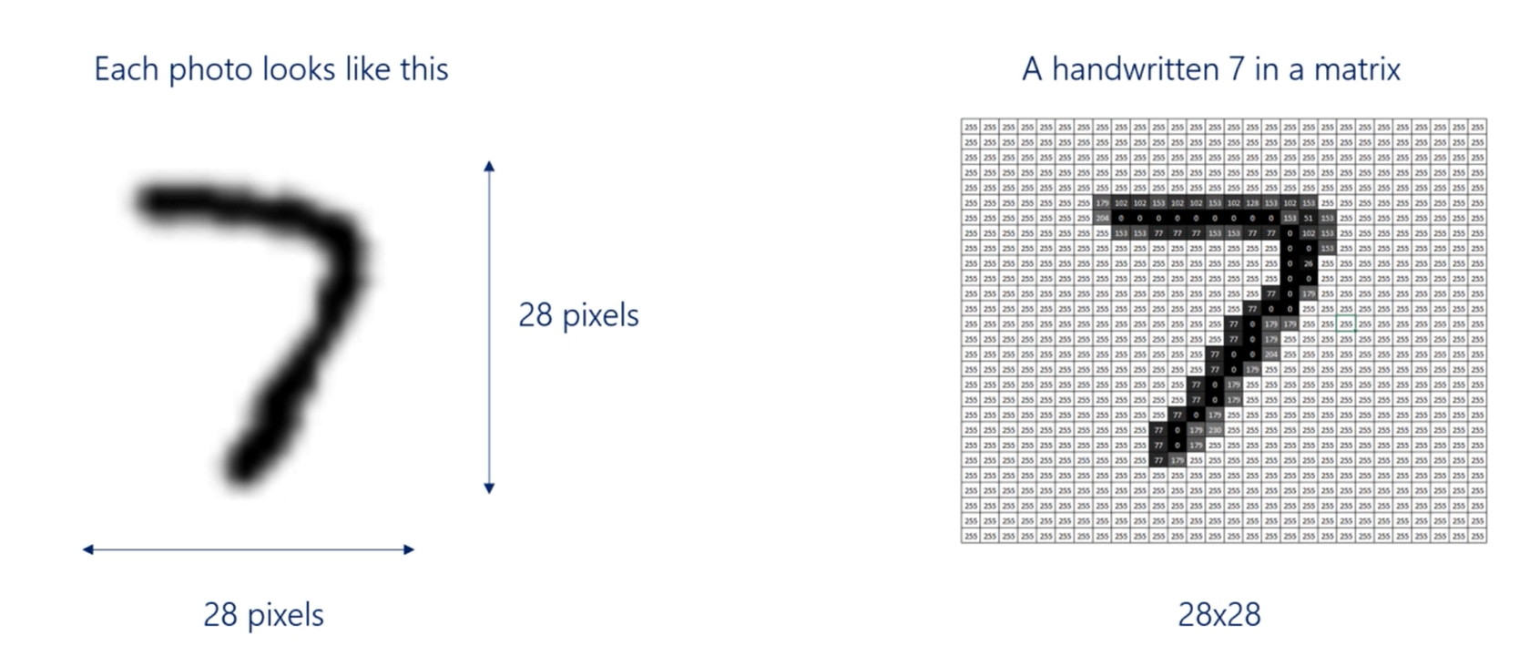
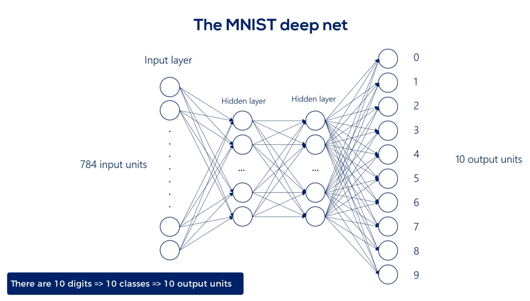
But the idea is more or less the same. Now because all the images are of the same size, a 28 by 28 photo will have 784 pixels.

The approach for deep feed forward neural networks is to transform or flatten each image into a vector of length 784, so for each image we would have 784 inputs.

Each input corresponds to the intensity of the color of the corresponding pixel.

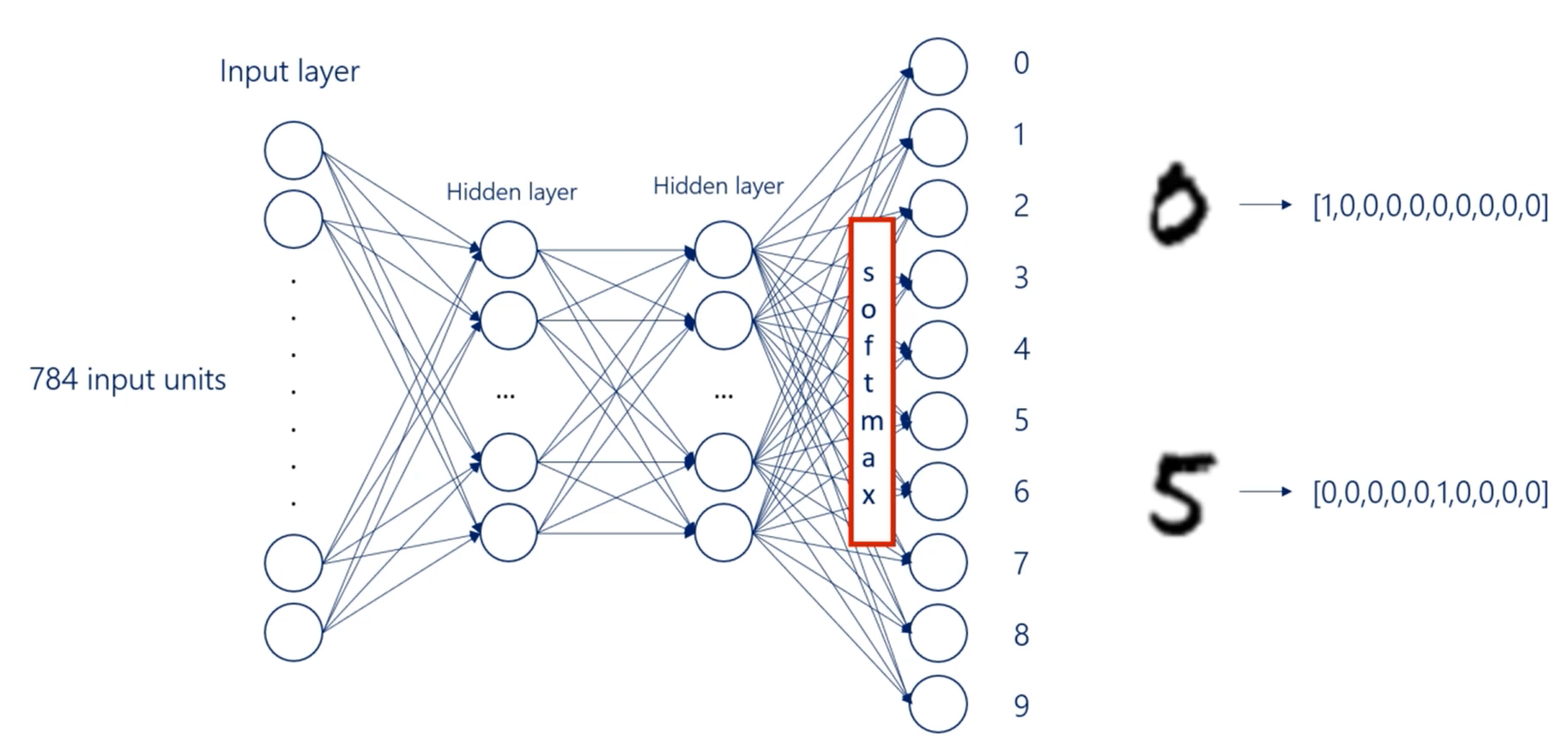
We will have 784 input units in our input layer, then we will linearly combine them and add a non linearity to get the first hidden layer.

For our example, We will build a model with two hidden layers. Two hidden layers are enough to produce a model with very good accuracy.

Finally, we will produce the output layer.

There are 10 digits so 10 classes.

Therefore, we will have 10 output units in the output layer

The utput will then be compared to the targets.

It will use one hot encoding for both the outputs and the targets.

For example, the digit 0 will be represented by this vector while the digit 5 by that one.

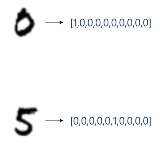
Since we would like to see the probability of a digit being rightfully labeled, we will use a soft Max activation function for the output layer.

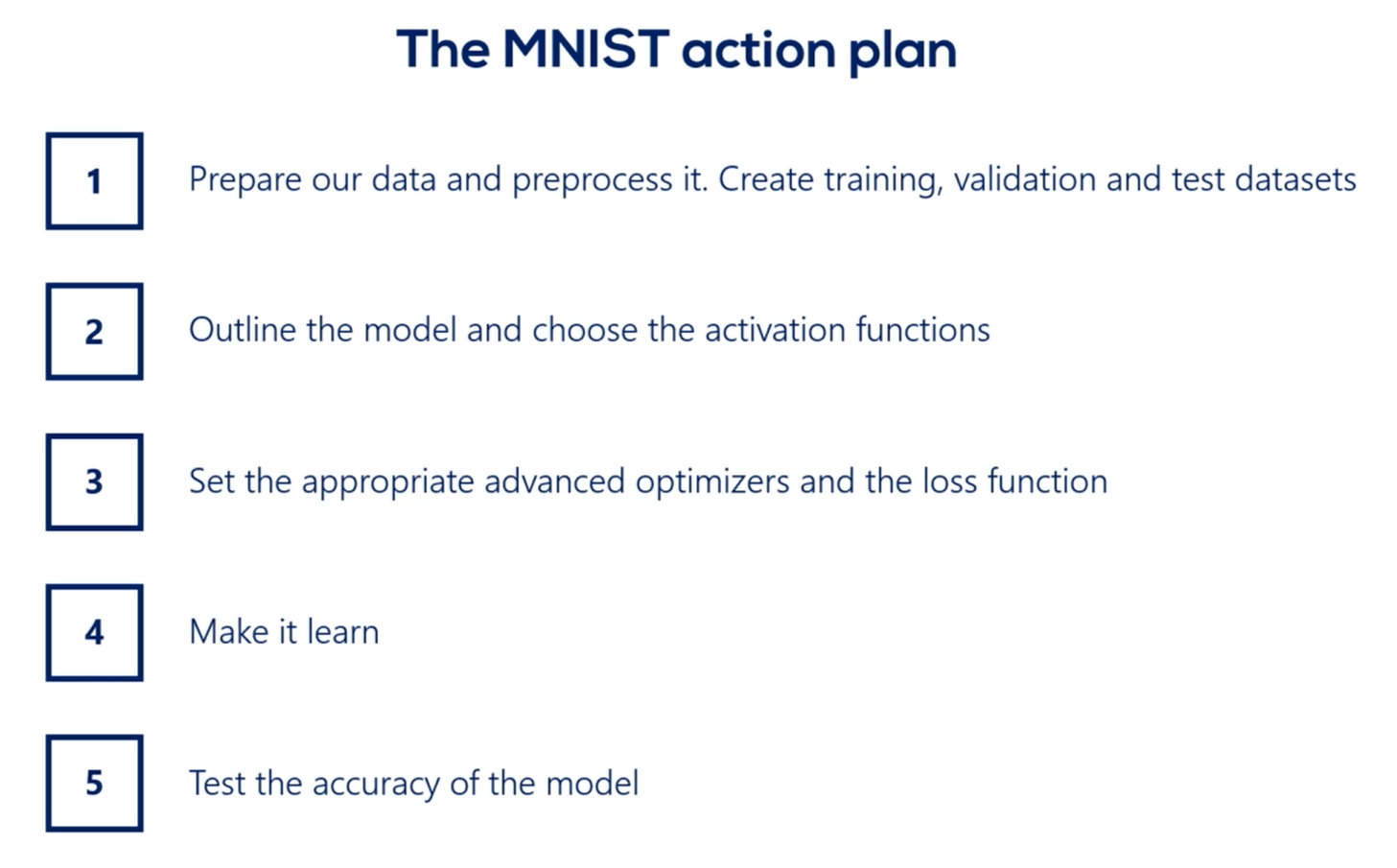
let's walk through the action plan.

1. First, we must prepare our data and pre process it a bit. We will create training validation and test data sets as well as select the batch size.

2. Second, we must outline the model and choose the activation functions we want to employ.

3. Third, we must set the appropriate advanced optimizers and the loss function.

4. Fourth, we will make it learn the algorithm will back propagate its way to accuracy at each epoch we will validate.

5. Finally, we will test the accuracy of the model regarding the test dataset.

MNIST example

Import the relevant packages

import numpy as np
import tensorflow as tf
import tensorflow_datasets as tfds

TIP

pip install tensorflow_datasets if pycharm doesn't have it in the project libraries to be installed.

Data

There are two tweaks we'd rather make.

First, we can set the argument as_supervised=True.

This will load the data set in a two tuple structure input and target.

In addition, let's include one final argument with_info=True and stored in the variable mnist_info.

This will provide us with a tuple containing information about the version, features, and number of samples of the dataset.

TIP

tfds.load(name, with_info, as_supervised) Loads a dataset from TensorFlow datasets .

-> as_supervised = Trues, loads the data in a 2-tuple structure [input,target]. -> with_info = True, provides a tuple containing info about version, features, #samples of the dataset

mnist_dataset, mnist_info = tfds.load(name='mnist', 
                                     with_info=True, 
                                     as_supervised=True)

Preprocessing the data

It's time to extract the train data and the test data.

Lucky for us, there are built in references that will help us achieve this.

mnist_train, mnist_test = mnist_dataset['train'], mnist_dataset['test']

Where is the Validation Dataset?

By default, TensorFlow MNIST has training and testing datasets, but no validation dataset.

Sure that's one of the more irritating properties of the tensor flow data sets module, but, in fact, it gives us the opportunity to actually practice splitting datasets on our own.

The train data set is much bigger than the test one. So we'll take our validation data from the train data set.

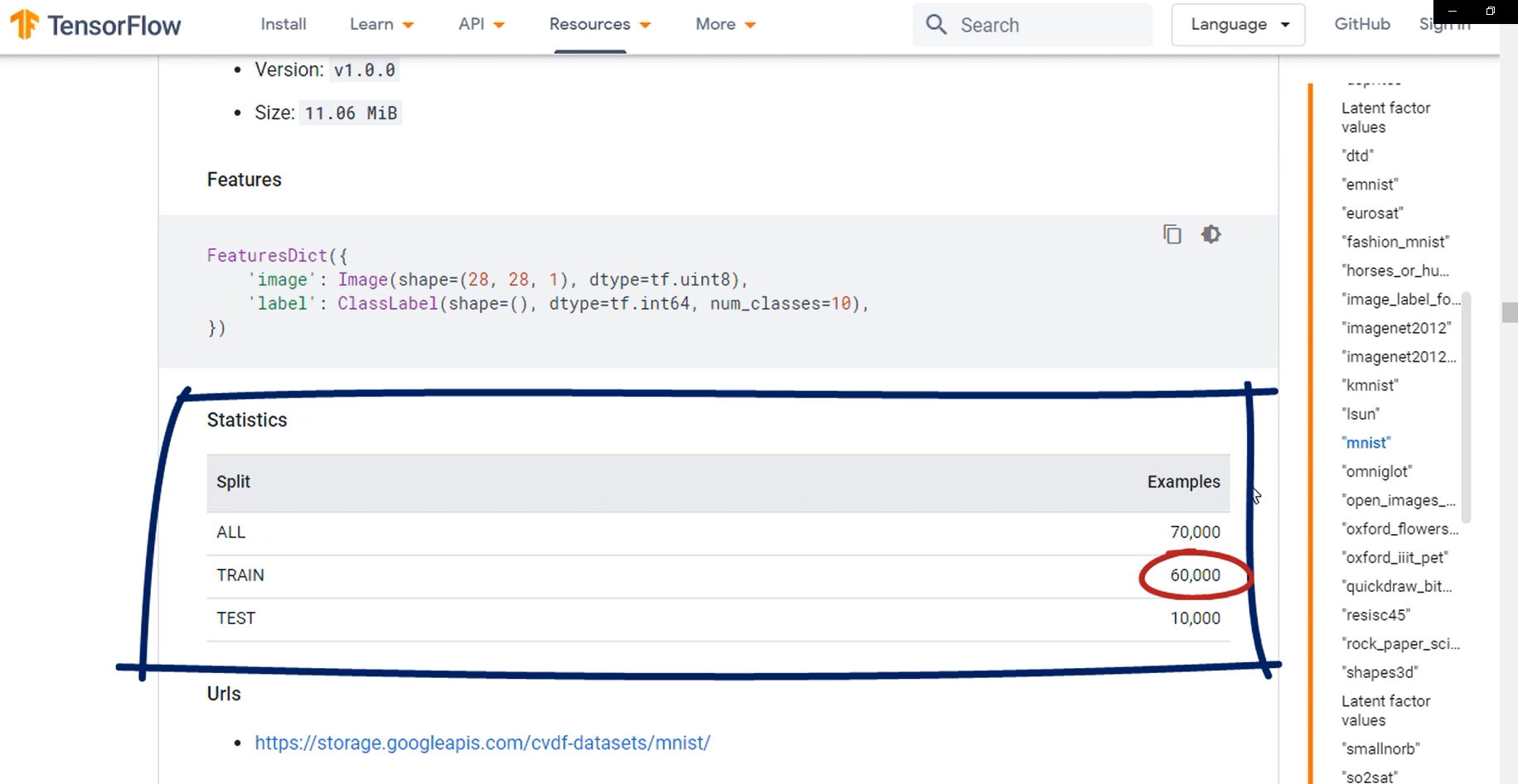
The easiest way to do that is to take an arbitrary percentage of the train data set to serve as validation. So let's take 10 percent of it.

We should start by setting the number of validation samples. We can either count the number of training samples, or we can use the amnesty info variable we've created earlier.

num_validation_samples = 0.1 * mnist_info.splits['train'].num_examples

OK, so we will get a number equal to the number of training samples divided by 10.

We are not sure that this will be an integer though, it may be 10000.2, which is not really a possible number of validation samples.

To solve this issue effortlessly, we can override the number of validation samples variable with:

num_validation_samples = tf.cast(num_validation_samples, tf.int64)

This will cast the value of stored in the number of validation samples variable to an integer, thereby preventing any potential issues.

Now, let's also store the number of test samples and a dedicated variable.

num_test_samples = mnist_info.splits['test'].num_examples
num_test_samples = tf.cast(num_test_samples, tf.int64)

Normally, we would also like to scale our data in some way to make the result more numerically stable.

In this case, we will simply prefer to have inputs between 0 and 1.

With that said, let's define a function that will scale the inputs called scale.

It will take an MNIST image and its label.

Let's make sure all values are floats so we will cast the image local variable to a float 32.

Next, we'll proceed by scaling it. As we already discussed the MNIST images contain values from 0 to 255 representing the 256 shades of gray.

Therefore, if we divide each element by 255 we'll get the desired result. All elements will be between 0 and 1.

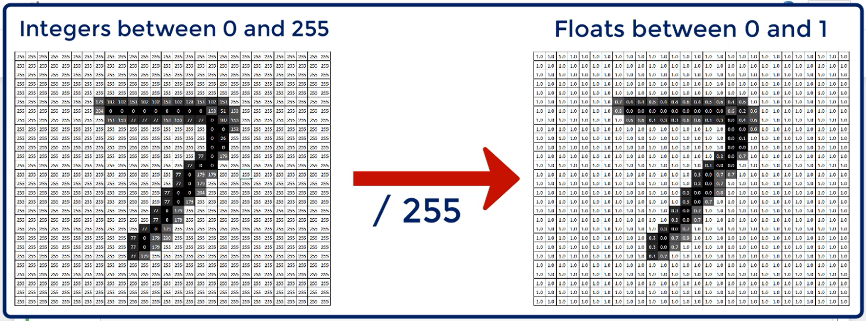
the dot at the end, once again, signifies that we want a result to be a float.

def scale(image, label):
    image = tf.cast(image, tf.float32)
    image /= 255.
    return image, label

So, this was a very specific function to write right?

In fact there is a TensorFlow method called map, which allows us to apply a custom transformation to a given dataset.

Moreover, this map can only apply transformations that can take an input and a label and return an input and a label.

That's what we build our scale function this way.

Note that you can scale your data in other ways if you see fit.

Just make sure that the function takes image and label and returns image and label. Thus you are simply transforming the values.

We've already decided we will take the validation data from MNIST train so:

This will scale the whole train dataset and store it in our new variable.

scaled_train_and_validation_data = mnist_train.map(scale)
test_data = mnist_test.map(scale)

Shuffling

In this lecture will first shuffle our data and then create the validation dataset. Shuffling is a little trick we like to apply in the pre processing stage.

When shuffling we are basically keeping the same information, but in a different order.

It's possible that the targets are stored in ascending order resulting in the first X batches having only 0 targets and the other batches having only 1 as a Target.

Since we'll be batching we'd better shuffle the data, it should be as randomly spread as possible, so that batching works as intended.

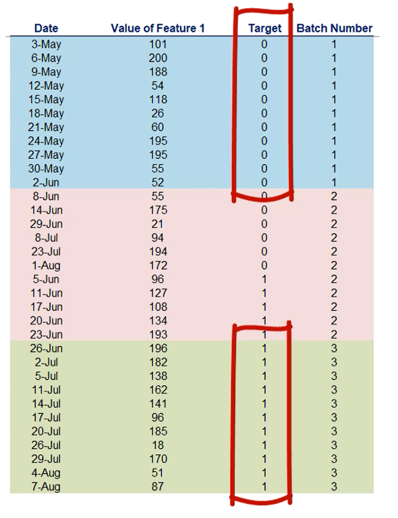
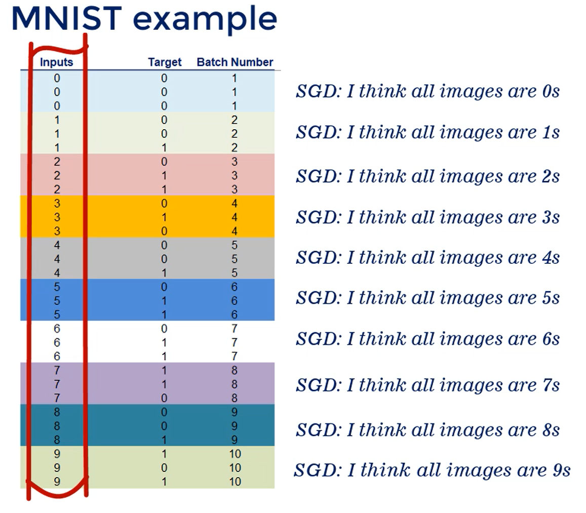
Let me give you an unrelated example.

Imagine the data is ordered and we have 10 batches each batch contains only a given digit.

So the first batch has only zeros, the second only ones the third only twos etc..

This will confuse the stochastic gradient descent algorithm, because each batch is homogenous inside it but completely different from all other batches, causing the loss to differ greatly.

In other words, we want the data shuffled.

OK we should start by defining a buffer size, to say, 10000.

BUFFER_SIZE = 10000

This buffer size parameter is used in cases when we are dealing with enormous datasets.

In such cases, we can't shuffle the whole data set in one go, because we can't possibly fit it all in the memory of the computer.

So, instead, we must instruct TensorFlow to take samples ten thousand at a time, shuffle them and then take the next ten thousand.

Logically, if we set the buffer size to twenty thousand, it will take twenty thousand samples at once.

Note that if the buffer size is equal to 1, no shuffling will actually happen.

So, if the buffer size is equal or bigger than the total number of samples shuffling will take place at once and shuffle them uniformly.

Finally, if we have a buffer size that's between one and the total sample size we'll be optimizing the computational power of our computer.

All right, time to do the shuffle.

Luckily for us, there is a shuffle method readily available, and we just need to specify the buffer size.

shuffled_train_and_validation_data = scaled_train_and_validation_data.shuffle(BUFFER_SIZE)

Once we have scaled and shuffle the data we can proceed to actually extracting the train and validation data sets.

Our validation data will be equal to 10 percent of the training set, which we have already calculated and stored in num_validation_samples.

We can use the method take() to extract that many samples.

validation_data = shuffled_train_and_validation_data.take(num_validation_samples)

We have successfully created a validation dataset.

In the same way we can create the train data by extracting all elements but the first X validation samples, an appropriate method here is skip().

train_data = shuffled_train_and_validation_data.skip(num_validation_samples)

We will be using Mini-batch gradient descent to train our model.

As we explained before, this is the most efficient way to perform deep learning, as the tradeoff between accuracy and speed is optimal.

To do that, we must set a batch size and prepare our data for batching.

Remember:

batch size = 1 = Stochastic gradient descent (SGD)

batch size = # samples = (single batch) GD

So, ideally we want:

1 < batch size < # samples = mini-batch GD

So, we want a number relatively small with regard to the data set but reasonably high. So what would allow us to preserve the underlying dependencies

let's set the BATCH_SIZE = 100. that's yet another hyper parameter that you may play with when you fine tune the algorithm.

There is a method batch we can use on the data set to combine its consecutive elements in the batches. Let's start with a train data we just created.

I'll simply overwrite it, as there is no need to preserve a version of this data that is not batched.

This will add a new column to our tensor that would indicate to the model how many samples it should take in each batch.

train_data = train_data.batch(BATCH_SIZE) 

What about the validation data?

Well, since we won't be back propagating on the validation data, but only forward propagating we don't really need to batch.

Remember that batching was useful in updating weights, only once per batch, which is like 100 samples rather than at every sample.

Hence, reducing noise in the training updates.

So, whenever we validate or test we simply forward propagate once. When batching, we usually find the average loss and average accuracy.

During validation and testing we want the exact values.

Therefore, we should take all the data at once.

Moreover, when forward propagating we don't use that much computational power so, it's not expensive to calculate the exact values.

However, the model expects our validation set in batch form too. That's why we should overwrite validation data with:

validation_data = validation_data.batch(num_validation_samples)

Here will have a single batch with a batch size equal to the total number of validation samples.

In this way, we'll create a new column in our tensor indicating that the model should take the whole validation dataset at once, when it utilizes it.

To handle our test data, we don't need to batch it either. We'll take the same approach we use with the validation set.

test_data = test_data.batch(num_validation_samples)

Finally, our validation data must have the same shape and object properties as the train and test data. The MNIST data is iterable and in 2-tuple format, as we set the argument as_supervised=True. Therefore, we must extract and convert the validation inputs and targets appropriately.

Let's store them in validation_inputs, validation_targets and set them to be equal to next(iter(validation_data)).

validation_inputs, validation_targets = next(iter(validation_data))

TIP

iter() creates an object which can be iterated one element at a time (e.g. in a for loop or while loop).

iter() is the python syntax for making the validation data an iterator.

By default, that will make the data set iterable, but will not load any data.

next() loads the next batch. Since there is only one batch, it will load the inputs and the targets.

Model

There are 784 inputs. So that's our input layer.

We have 10 outputs nodes one for each digit.

We will work with 2 hidden layers consisting of 50 nodes each.

As you may recall the width and the depth of the net are hyper parameters. I don't know the optimal width and depth for this problem but I surely know that what I've chosen right now is suboptimal.

Anyhow, in your next homework you'll have the chance to fine tune the hyper parameters of our model and obtain an improved result.

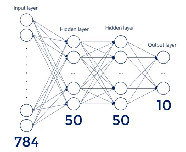
Homework

Test different Widths and Depths

All right, let's declare three variables for width of the inputs, outputs and hidden layers.

input_size = 784
output_size = 10
hidden_layer_size = 50

The underlying assumption is that all hidden layers are of the same size. Alternatively, you can create hidden layers with different width, and see if they work better for your problem.

Next, we must define the actual model.

Once again, we will store it in a variable called model.

The first layer is the input layer. Our data is such that each observation is 28 by 28 by 1 or a tensor of rank 3.

model = tf.keras.Sequential([])

As we already discussed, since we don't know CNN's we need to flatten the images into a vector.

Note that this is a common operation and deep learning, so there is a dedicated method called flatten.

flatten is a part of the layers module and takes his argument the shape of the object we want to flatten.

It transforms it, or more specifically flattens it, into a vector.

tf.keras.layers.Flatten(input_shape=(28, 28, 1))

Thus, we have prepared our data for a feed forward neural network of the same kind that we've discussed so far in the course.

The next step is building the neural network in a very similar way to our tensor flow intro model. We employ tf.keras.layers.Dense to build each consecutive layer.

TIP

Let me remind you that tf.keras.layers.Dense was, basically, finding the dot product of the inputs and weights and adding the bias.

Now let's build on that. It can apply an activation function to this expression. This is precisely what we've discussed so far theoretically, it's time to see how it is implemented.

tf.keras.layers.Dense takes his arguments the output size of the mathematical operation.

In this case, we are getting from the inputs to the first hidden layer.

Therefore, the output of the first mathematical operation will have the shape of the first hidden layer as a second argument.

We can include an activation function.

I'll go for re Lou because I know it works very well for this problem.

In practice, each neural network has a different optimal combination of activation functions.

tf.keras.layers.Dense(hidden_layer_size, activation='relu'),

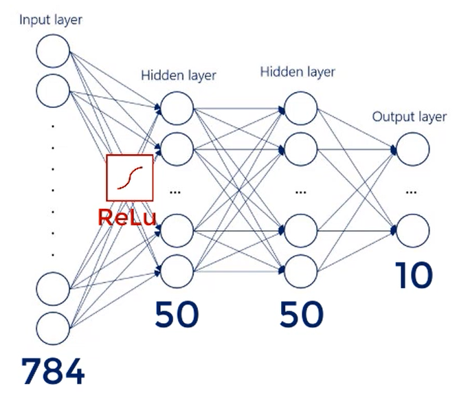
Homework

Test different activation functions

So far, we've got our flattened inputs and the first hidden layer, we can create the second hidden layer in the same way.

tf.keras.layers.Dense(hidden_layer_size, activation='relu'),

TIP

Add another layer here to increase the depth of the neural network.

The final layer is the output layer.

It is no different in terms of syntax.

As you've probably guessed we use the dense to create it.

This time though, we specify the output size rather than the hidden layer size, as we can see from the diagram.

What about the activation?

Well, from the theoretical lessons you know that when we are creating a classifier the activation function of the output layer must transform the values into probabilities.

Therefore, we must opt for the SoftMax.

tf.keras.layers.Dense(output_size, activation='softmax'), 

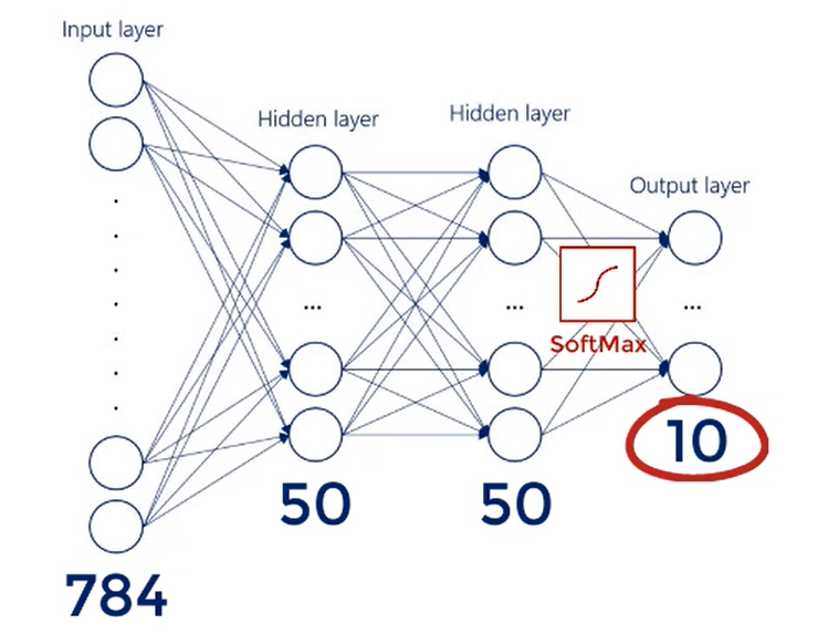
That's all our model has been built.

input_size = 784
output_size = 10
hidden_layer_size = 50

model = tf.keras.Sequential([
        tf.keras.layers.Flatten(input_shape=(28, 28, 1)),
        tf.keras.layers.Dense(hidden_layer_size, activation='relu'),
        tf.keras.layers.Dense(hidden_layer_size, activation='relu'),
        tf.keras.layers.Dense(output_size, activation='softmax'), 
        ])

Next step, The optimization algorithm.

Choose the optimizer and the loss function

We've taken care of the data and the model.

Now, let's proceed with the next essential steps.

Similar to our tensor flow intro lecture, we must specify the optimizer and the loss through the compile method we call on the model object.

We start by specifying the optimizer, we know that one of the best choices we've got is the adaptive moment estimation or Adam in short.

As you may recall, TensorFlow allows us to use a string to define the optimizer. We simply write adam, by the way, these strings are not case sensitive so you can capitalize the first letter or all letters if you wish.

model.compile(optimizer='adam')

What about the loss function?

Well, we'd like to employ a loss that is used for classifiers price.

Entropy would normally be our first choice.

However, there are different types of cross entropy in tensor flow too.

There are three built in variations of across entropy loss.

• binary_crossentropy
• categorical_crossentropy
• sparse_categorical_crossentropy

binary_crossentropy refers to the case where we've got binary encoding, so we won't be choosing this one.

categorical_crossentropy and sparse_categorical_crossentropy are equivalent, with the difference that sparse_categorical_crossentropy applies one-hot encoding to the data.

Is our data one-hot encoded?

Well, that was not a pre processing step we went through, however, the output in the target layer should have matching forms, our model and optimizer expect the output shape to match the target shape in a one-hot encoded format.

This means we should opt for the sparse_categorical_crossentropy.

model.compile(optimizer='adam', loss='sparse_categorical_crossentropy')

Finally, we can add a third argument to compile.

We could include metrics that we wish to calculate throughout the training and testing processes.

Typically, that's the accuracy. So let's add it here.

model.compile(optimizer='adam',
              loss='sparse_categorical_crossentropy',
              metrics=['accuracy'])

Training

We've reached the most exciting part of the machine learning process training. This is where we fit the model we have built and see if it actually works so to speak first let's create a variable storing the number of epochs that we wish to train for.

I'll call it NUM_EPOCHS and arbitrarily set it to 5.

NUM_EPOCHS = 5

Next, we can fit the model similar to our TensorFlow intro. We will use the fit() method so, model.fit(). First we specify the data. In this case train_data. Second, we set the number of epochs NUM_EPOCHS.

TIP

Note that we have parameterize it in a neat way, so we can clearly inspect and amend the number of epochs.

Whenever we have hyper parameters such as the buffer_size, batch_size, input_size, output_size and so on, We prefer to create dedicated variables, that can be easily spotted when we fine tune or debug our code.

model.fit(train_data, epochs=NUM_EPOCHS)

This alone would be enough to train the model. However, we also need to validate. It's a good thing we've already prepared the validation_data, what we have to do now is include it as an argument, that same method equal to the validation_inputs and validation_targets we created earlier.

model.fit(train_data, epochs=NUM_EPOCHS, validation_data=(validation_inputs, validation_targets))

Finally, I'll set verbose=2 to make sure we receive only the most important information for each epoch.

model.fit(train_data, epochs=NUM_EPOCHS, validation_data=(validation_inputs, validation_targets), verbose=2)

Let's briefly explain what we expect to happen behind the curtains.

1. At the beginning of each epoch, the training loss will be set to zero.

2. The algorithm will iterate over a preset number of batches, all extracted from the training set. Essentially, the whole training set will be utilized, but in batches.

3. Therefore, the weights and biases will be updated as many times as there are batches.

4. At the end of each epoch, we'll get a value for the lost function, indicating how the training is going.

5. Moreover, we'll also see a training accuracy, thanks to the last argument we added.

6. Then, at the end of the epoch, the algorithm will forward propagate the whole validation data set in a single batch through the optimized model and calculate the validation accuracy.

7. When we reach the maximum number of epochs the training will be over.

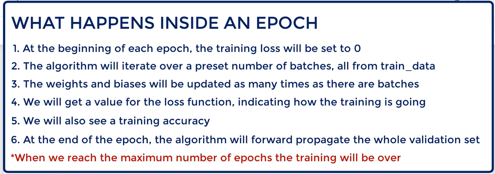
Let's run the code:

What we see are several lines of output.

First, we have information about the number of the epoch, Epoch 1/5.

Next, we've got the number of batches. It says 540 out of 540, because if we had a progress bar that would fill out gradually.

The third piece of information is the time it took for the epoch to conclude, around one to two seconds per epoch. 2s

Next, we can see the training loss.

It doesn't make sense to investigated separately. It should be compared to the training loss across epochs. In this case it is mostly decreasing.

loss: 0.4242 --> 0.1926 --> 0.1426 --> 0.1144 --> 0.0963

Note that it didn't change too much, because even after the first epoch we've already had 540 different weight and bias updates, one for each batch.

What follows is the accuracy, which shows what percent of the cases our output were equal to the targets.

Logically, it follows the trend of the loss. After all, they both represent how well the outputs match the targets.

accuracy: 0.8829 --> 0.9443 --> 0.9580 --> 0.9669 --> 0.9706

Finally, we've got the loss and the accuracy for the validation dataset. They are our check.

We usually keep an eye on the validation loss to determine whether the model is overfitting. The validation accuracy on the other hand is the true accuracy of the model for the epoch.

This is because the training accuracy is the average accuracy across batches. While the validation accuracy is that of the whole validation set.

Epoch 1/5
540/540 - 2s - loss: 0.4242 - accuracy: 0.8829 - val_loss: 0.2248 - val_accuracy: 0.9385
Epoch 2/5
540/540 - 1s - loss: 0.1926 - accuracy: 0.9443 - val_loss: 0.1681 - val_accuracy: 0.9517
Epoch 3/5
540/540 - 1s - loss: 0.1426 - accuracy: 0.9580 - val_loss: 0.1433 - val_accuracy: 0.9568
Epoch 4/5
540/540 - 1s - loss: 0.1144 - accuracy: 0.9669 - val_loss: 0.1095 - val_accuracy: 0.9665
Epoch 5/5
540/540 - 1s - loss: 0.0963 - accuracy: 0.9706 - val_loss: 0.0919 - val_accuracy: 0.9735

To assess the overall accuracy of our model we look at the validation accuracy for the last debunk. val_accuracy: 0.9735 For us it's a 97.35%. This is a remarkable result.

Can we do better?

Let's try fiddling a bit with the model.

We can change many of the hyper parameters, but I'll start from the hidden layer size instead of 50 nodes in each set in layer, let's go for 100.

input_size = 784
output_size = 10
hidden_layer_size = 100

model = tf.keras.Sequential([
                            tf.keras.layers.Flatten(input_shape=(28, 28, 1)),
                            tf.keras.layers.Dense(hidden_layer_size, activation='relu'),
                            tf.keras.layers.Dense(hidden_layer_size, activation='relu'),
                            tf.keras.layers.Dense(output_size, activation='softmax'),
                            ])

running the code we have:

Epoch 1/5
540/540 - 1s - loss: 0.3340 - accuracy: 0.9051 - val_loss: 0.1651 - val_accuracy: 0.9522
Epoch 2/5
540/540 - 1s - loss: 0.1388 - accuracy: 0.9589 - val_loss: 0.1109 - val_accuracy: 0.9680
Epoch 3/5
540/540 - 1s - loss: 0.0956 - accuracy: 0.9708 - val_loss: 0.0866 - val_accuracy: 0.9737
Epoch 4/5
540/540 - 1s - loss: 0.0761 - accuracy: 0.9768 - val_loss: 0.0774 - val_accuracy: 0.9757
Epoch 5/5
540/540 - 1s - loss: 0.0610 - accuracy: 0.9810 - val_loss: 0.0680 - val_accuracy: 0.9778

Including TensorBoard

To include TensorBoard we have to include:

import time
from tensorflow.keras.callbacks import TensorBoard

NAME = "LinearRegression-{}".format(int(time.time()))
tensorboard = TensorBoard(log_dir='logs/{}'.format(NAME))

Then, on the model.fit, we include the TensorBoard callback:

model.fit(train_data, epochs=NUM_EPOCHS, validation_data=(validation_inputs, validation_targets), verbose=2, callbacks=[tensorboard])

After we execute the model we can go the the terminal and call:

tensorboard --logdir logs/

Here are the results:

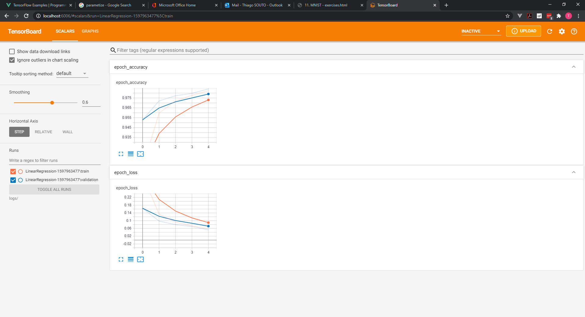
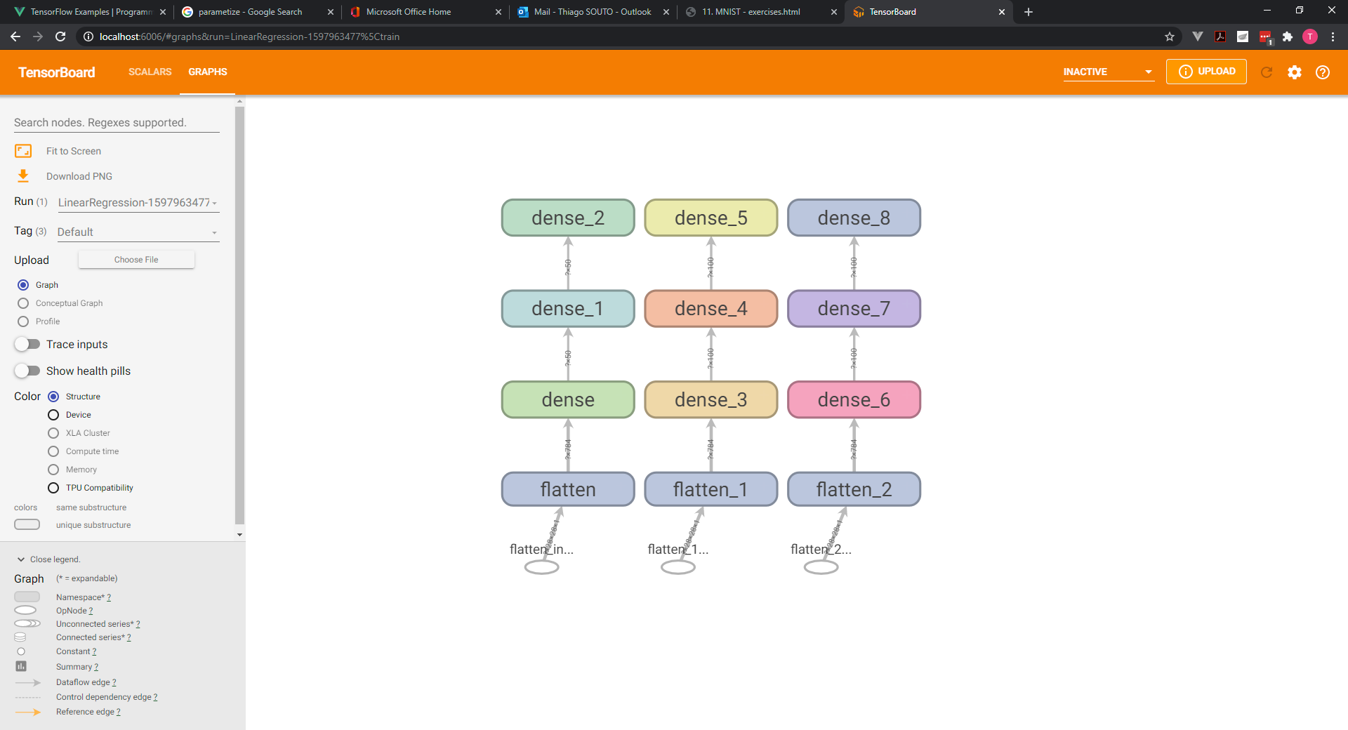
Epoch Loss:

Epoch Accuracy:

Now we have val_accuracy: 0.9778 or 97.78%

Improving the model

There are several main adjustments you may try.

Please pay attention to the time it takes for each epoch to conclude.

Using the code from the lecture as the basis, fiddle with the hyperparameters of the algorithm.

1. The width (the hidden layer size) of the algorithm. Try a hidden layer size of 200. How does the validation accuracy of the model change? What about the time it took the algorithm to train? Can you find a hidden layer size that does better?

Epoch 1/5
540/540 - 2s - loss: 0.2666 - accuracy: 0.9219 - val_loss: 0.1214 - val_accuracy: 0.9672
Epoch 2/5
540/540 - 2s - loss: 0.1046 - accuracy: 0.9689 - val_loss: 0.0802 - val_accuracy: 0.9763
Epoch 3/5
540/540 - 2s - loss: 0.0696 - accuracy: 0.9791 - val_loss: 0.0657 - val_accuracy: 0.9788
Epoch 4/5
540/540 - 2s - loss: 0.0519 - accuracy: 0.9836 - val_loss: 0.0488 - val_accuracy: 0.9852
Epoch 5/5
540/540 - 2s - loss: 0.0396 - accuracy: 0.9876 - val_loss: 0.0533 - val_accuracy: 0.9835

Now we have val_accuracy: 0.9835 or 98.35%

Epoch Loss:

Epoch Accuracy:

2. The depth of the algorithm. Add another hidden layer to the algorithm. This is an extremely important exercise! How does the validation accuracy change? What about the time it took the algorithm to train? Hint: Be careful with the shapes of the weights and the biases.

Now we have val_accuracy: 0.9857 or 98.57%

Epoch 1/5
540/540 - 2s - loss: 0.2645 - accuracy: 0.9221 - val_loss: 0.1256 - val_accuracy: 0.9650
Epoch 2/5
540/540 - 2s - loss: 0.1040 - accuracy: 0.9682 - val_loss: 0.0742 - val_accuracy: 0.9793
Epoch 3/5
540/540 - 2s - loss: 0.0710 - accuracy: 0.9779 - val_loss: 0.0665 - val_accuracy: 0.9797
Epoch 4/5
540/540 - 2s - loss: 0.0516 - accuracy: 0.9827 - val_loss: 0.0416 - val_accuracy: 0.9868
Epoch 5/5
540/540 - 2s - loss: 0.0408 - accuracy: 0.9866 - val_loss: 0.0471 - val_accuracy: 0.9857

Epoch Loss:

Epoch Accuracy:

3. The width and depth of the algorithm. Add as many additional layers as you need to reach 5 hidden layers. Moreover, adjust the width of the algorithm as you find suitable. How does the validation accuracy change? What about the time it took the algorithm to train?

Now we have val_accuracy: 0.9877 or 98.77%

Epoch 1/5
540/540 - 3s - loss: 0.2552 - accuracy: 0.9216 - val_loss: 0.1033 - val_accuracy: 0.9705
Epoch 2/5
540/540 - 3s - loss: 0.1062 - accuracy: 0.9683 - val_loss: 0.0970 - val_accuracy: 0.9730
Epoch 3/5
540/540 - 3s - loss: 0.0727 - accuracy: 0.9780 - val_loss: 0.0663 - val_accuracy: 0.9800
Epoch 4/5
540/540 - 3s - loss: 0.0588 - accuracy: 0.9823 - val_loss: 0.0770 - val_accuracy: 0.9787
Epoch 5/5
540/540 - 3s - loss: 0.0504 - accuracy: 0.9849 - val_loss: 0.0508 - val_accuracy: 0.9877

Epoch Loss:

Epoch Accuracy:

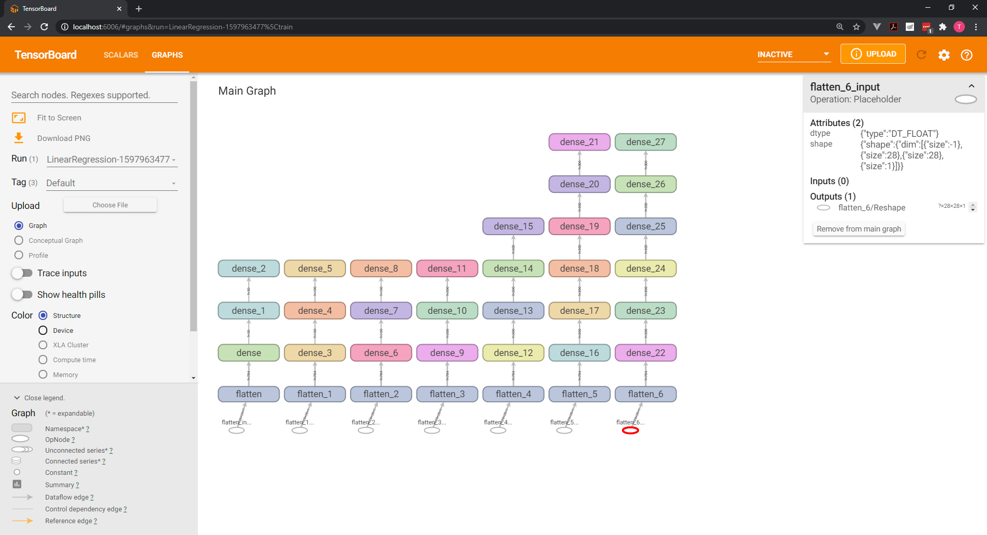
4. Fiddle with the activation functions. Try applying sigmoid transformation to both layers. The sigmoid activation is given by the string 'sigmoid'.

With the sigmoid in all layers It doesn't improved the model:

Epoch 1/5
540/540 - 3s - loss: 1.1286 - accuracy: 0.5806 - val_loss: 0.3802 - val_accuracy: 0.8875
Epoch 2/5
540/540 - 3s - loss: 0.3112 - accuracy: 0.9095 - val_loss: 0.2120 - val_accuracy: 0.9382
Epoch 3/5
540/540 - 3s - loss: 0.1960 - accuracy: 0.9431 - val_loss: 0.1641 - val_accuracy: 0.9523
Epoch 4/5
540/540 - 3s - loss: 0.1470 - accuracy: 0.9569 - val_loss: 0.1225 - val_accuracy: 0.9640
Epoch 5/5
540/540 - 3s - loss: 0.1155 - accuracy: 0.9662 - val_loss: 0.0995 - val_accuracy: 0.9727

5. Fiddle with the activation functions. Try applying a ReLu to the first hidden layer and tanh to the second one. The tanh activation is given by the string 'tanh'.

Best configuration so far:

Now we have val_accuracy: 0.9882 or 98.82%

Epoch 1/5
540/540 - 2s - loss: 0.2323 - accuracy: 0.9299 - val_loss: 0.1038 - val_accuracy: 0.9700
Epoch 2/5
540/540 - 2s - loss: 0.0870 - accuracy: 0.9734 - val_loss: 0.0645 - val_accuracy: 0.9822
Epoch 3/5
540/540 - 2s - loss: 0.0605 - accuracy: 0.9808 - val_loss: 0.0534 - val_accuracy: 0.9850
Epoch 4/5
540/540 - 2s - loss: 0.0419 - accuracy: 0.9870 - val_loss: 0.0476 - val_accuracy: 0.9870
Epoch 5/5
540/540 - 2s - loss: 0.0354 - accuracy: 0.9884 - val_loss: 0.0363 - val_accuracy: 0.9882

6. Adjust the batch size. Try a batch size of 10000. How does the required time change? What about the accuracy?

With batch size of 10000 the model didn't improve:

Now we have val_accuracy: 0.9177 or 91.77%

Epoch 1/5
6/6 - 3s - loss: 1.7442 - accuracy: 0.5264 - val_loss: 0.9509 - val_accuracy: 0.8043
Epoch 2/5
6/6 - 1s - loss: 0.7309 - accuracy: 0.8264 - val_loss: 0.4965 - val_accuracy: 0.8613
Epoch 3/5
6/6 - 1s - loss: 0.4381 - accuracy: 0.8762 - val_loss: 0.3754 - val_accuracy: 0.8872
Epoch 4/5
6/6 - 1s - loss: 0.3481 - accuracy: 0.8972 - val_loss: 0.3191 - val_accuracy: 0.9035
Epoch 5/5
6/6 - 1s - loss: 0.2971 - accuracy: 0.9110 - val_loss: 0.2803 - val_accuracy: 0.9177

7. Adjust the batch size. Try a batch size of 1. That's the SGD. How do the time and accuracy change? Is the result coherent with the theory?

With the batch size of 1 the time for the epochs were much longer, and the model didn't improved.

Epoch 1/5
54000/54000 - 52s - loss: 0.2705 - accuracy: 0.9248 - val_loss: 0.1855 - val_accuracy: 0.9512
Epoch 2/5
54000/54000 - 56s - loss: 0.1652 - accuracy: 0.9585 - val_loss: 0.1752 - val_accuracy: 0.9572
Epoch 3/5
54000/54000 - 79s - loss: 0.1414 - accuracy: 0.9654 - val_loss: 0.1279 - val_accuracy: 0.9678
Epoch 4/5
54000/54000 - 86s - loss: 0.1325 - accuracy: 0.9674 - val_loss: 0.1864 - val_accuracy: 0.9522
Epoch 5/5
54000/54000 - 92s - loss: 0.1255 - accuracy: 0.9689 - val_loss: 0.1363 - val_accuracy: 0.9702

8. Adjust the learning rate. Try a value of 0.0001. Does it make a difference?

To adjust the learning rate we can:

custom_optimizer = tf.keras.optimizers.Adam(learning_rate=0.02)

model.compile(optimizer=custom_optimizer, loss='sparse_categorical_crossentropy', metrics=['accuracy'])

BATCH_SIZE = 100 was set.

Epoch 1/5
540/540 - 4s - loss: 0.3102 - accuracy: 0.9206 - val_loss: 0.2927 - val_accuracy: 0.9263
Epoch 2/5
540/540 - 3s - loss: 0.2815 - accuracy: 0.9264 - val_loss: 0.2796 - val_accuracy: 0.9263
Epoch 3/5
540/540 - 3s - loss: 0.2726 - accuracy: 0.9284 - val_loss: 0.2722 - val_accuracy: 0.9295
Epoch 4/5
540/540 - 3s - loss: 0.2625 - accuracy: 0.9307 - val_loss: 0.2650 - val_accuracy: 0.9307
Epoch 5/5
540/540 - 3s - loss: 0.2529 - accuracy: 0.9321 - val_loss: 0.2586 - val_accuracy: 0.9317

TIP

For Adam, the Defaults learning rate is 0.001.

9. Adjust the learning rate. Try a value of 0.02. Does it make a difference?

Epoch 1/5
540/540 - 4s - loss: 0.3852 - accuracy: 0.9076 - val_loss: 0.4712 - val_accuracy: 0.8845
Epoch 2/5
540/540 - 3s - loss: 0.3893 - accuracy: 0.9068 - val_loss: 0.3210 - val_accuracy: 0.9182
Epoch 3/5
540/540 - 3s - loss: 0.4046 - accuracy: 0.9013 - val_loss: 0.3917 - val_accuracy: 0.9002
Epoch 4/5
540/540 - 3s - loss: 0.4027 - accuracy: 0.8984 - val_loss: 0.4648 - val_accuracy: 0.8865
Epoch 5/5
540/540 - 3s - loss: 0.4337 - accuracy: 0.8947 - val_loss: 0.4309 - val_accuracy: 0.8948

10. Combine all the methods above and try to reach a validation accuracy of 98.5+ percent.

Best result: 98.88%

• BATCH_SIZE = 100
• Adam with default learning rate
• 2 Layers with relu and tanh - Depth
• hidden_layer_size = 300

Epoch 1/5
540/540 - 3s - loss: 0.2273 - accuracy: 0.9324 - val_loss: 0.1172 - val_accuracy: 0.9658
Epoch 2/5
540/540 - 2s - loss: 0.0899 - accuracy: 0.9728 - val_loss: 0.0758 - val_accuracy: 0.9773
Epoch 3/5
540/540 - 2s - loss: 0.0590 - accuracy: 0.9811 - val_loss: 0.0535 - val_accuracy: 0.9822
Epoch 4/5
540/540 - 2s - loss: 0.0415 - accuracy: 0.9866 - val_loss: 0.0463 - val_accuracy: 0.9840
Epoch 5/5
540/540 - 2s - loss: 0.0327 - accuracy: 0.9891 - val_loss: 0.0360 - val_accuracy: 0.9888

import tensorflow as tf
import tensorflow_datasets as tfds

import time
from tensorflow.keras.callbacks import TensorBoard

NAME = "LinearRegression-5Layers-300width-{}".format(int(time.time()))
tensorboard = TensorBoard(log_dir='logs/{}'.format(NAME))

#%%
# loading the data
mnist_dataset, mnist_info = tfds.load(name='mnist', with_info=True, as_supervised=True)


#%%
# Preprocessing the data
# Dividing into two sets
mnist_train, mnist_test = mnist_dataset['train'], mnist_dataset['test']

# setting the number of validation samples as 10% of the train dataset
num_validation_samples = 0.1 * mnist_info.splits['train'].num_examples

# override the number of validation samples variable to make it an integer
num_validation_samples = tf.cast(num_validation_samples, tf.int64)

# same process for test samples
num_test_samples = mnist_info.splits['test'].num_examples
num_test_samples = tf.cast(num_test_samples, tf.int64)

# scale the data to make the result more numerically stable.
def scale(image, label):
    image = tf.cast(image, tf.float32)
    image /= 255.
    return image, label

# Scale the whole train dataset and store it in our new variable.
scaled_train_and_validation_data = mnist_train.map(scale)
test_data = mnist_test.map(scale)

BUFFER_SIZE = 10000

shuffled_train_and_validation_data = scaled_train_and_validation_data.shuffle(BUFFER_SIZE)

validation_data = shuffled_train_and_validation_data.take(num_validation_samples)

train_data = shuffled_train_and_validation_data.skip(num_validation_samples)

BATCH_SIZE = 100

train_data = train_data.batch(BATCH_SIZE)

validation_data = validation_data.batch(num_validation_samples)

test_data = test_data.batch(num_validation_samples)

validation_inputs, validation_targets = next(iter(validation_data))




#%%
input_size = 784
output_size = 10
hidden_layer_size = 300

model = tf.keras.Sequential([
                            tf.keras.layers.Flatten(input_shape=(28, 28, 1)),
                            tf.keras.layers.Dense(hidden_layer_size, activation='relu'),
                            tf.keras.layers.Dense(hidden_layer_size, activation='tanh'),
                            tf.keras.layers.Dense(output_size, activation='softmax'),
                            ])

#%%
# Choose the optimizer and loss function

model.compile(optimizer='adam', loss='sparse_categorical_crossentropy', metrics=['accuracy'])


#%%
# Training

NUM_EPOCHS = 5

model.fit(train_data, epochs=NUM_EPOCHS, validation_data=(validation_inputs, validation_targets), verbose=2, callbacks=[tensorboard])

Test the model

We must still test the model on the test data set, because the final accuracy of the model comes from forward propagating the test dataset not the validation.

The reason is, we may have overfitted it. But didn't we already deal with overfishing ? That's a fine point, as some of you could miss the difference between validation and test datasets. So let's clarify that.

We train on the training data and then validate on the validation data.

That's how we make sure our parameters the weights and the biases don't over fit.

Once we train our first model though, we fiddle with the hyper parameters, normally we won't change only the width of the hidden layers. We can adjust the depth, the learning rate, the batch size, the activation functions for each layer and so on.

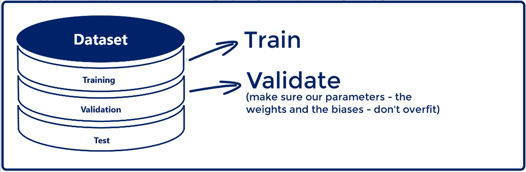
Each time we make a change, we run the model once more and check out the validation accuracy improved, after 10 to 20 different combinations, we may reach a model without standing validation accuracy.

In essence, we are trying to find the best hyper parameters. But what we find are not the best hyper parameters in general. These are the hyper parameters that fit our validation data set best, basically, by fine tuning them we are overfitting the validation data set.

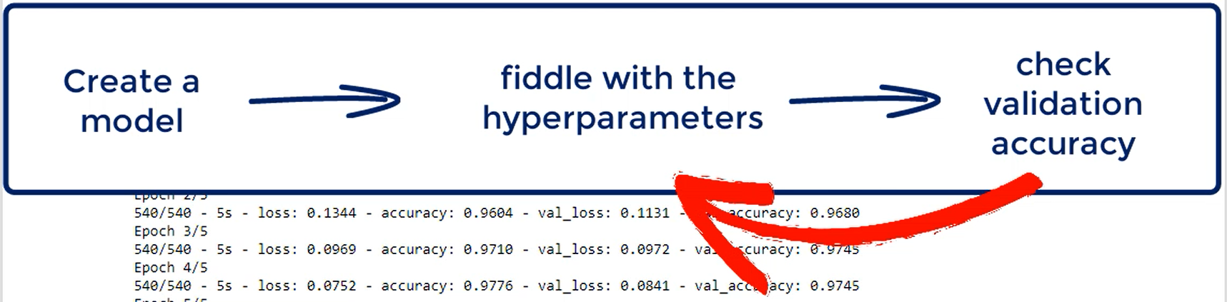
Let's elaborate a bit:

During the training stage, We can over fit the parameters or the weights and biases.

The validation data set is our reality check, that prevents us from overfitting the parameters.

After fiddling with the hyper parameters, we can over fit the validation data set, as we are considering the validation accuracy as a benchmark for how good the model is.

The test data set then, is our reality check, that prevents us from over fitting the hyper parameters. It is a data set the model has truly never seen.

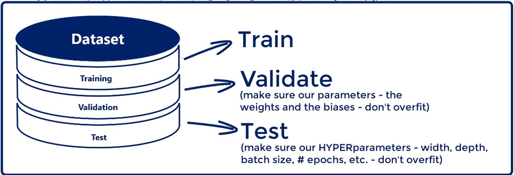
Let's test the model then, we can assess the test accuracy using the method evaluate().

So if we write model.evaluate(test_data) we will be forward propagating the test data through the net.

With our current model structure, there would be two outputs the loss and the accuracy. The same ones we had in the training stage.

To make it clearer, I'll store them in test_loss and test_accuracy.

test_loss, test_accuracy = model.evaluate(test_data)

To display them we can do:

print('Test loss: {0:.2f}. Test accuracy: {1:.2f}%.'.format(test_loss, test_accuracy*100.))

And we have:

Test loss: 0.07. Test accuracy: 97.95%.

Our model has a final test accuracy around 97.95%. This is also the final stage of the machine learning process.

After we test the model, conceptually we are no longer allowed to change it.

If you start changing the model after this point, the test data will no longer be a data set the model has never seen.

You'd have feedback that it has around 97.95% accuracy with this particular configuration.

The main point of the test dataset is to simulate model deployment if we get 50 percent or 60 percent testing accuracy, we will know for sure that our model has over fit, and it will fail miserably in real life.

However, getting a value very close to the validation accuracy shows that we have not over fit.

Finally, the test accuracy is the accuracy we expect to observe if we deploy the model in the real world.

Business Case

Our task is simple create a machine learning algorithm that can predict if a customer will buy again.

This is a classification problem with two classes: won't buy and will buy, represented by 0 and 1.

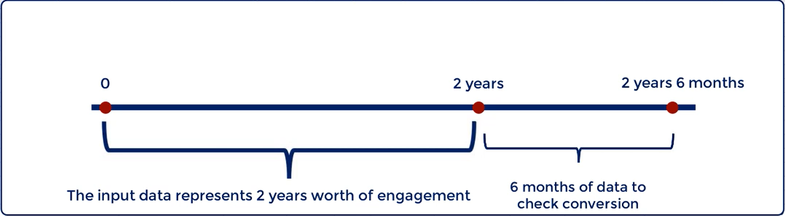
Outlining the business case solution

Since we are working with real life data, we must preprocess it, this is important for machine learning in a data science team. There may be a person whose sole job is to prepare data sets for analysis.

This is why we would like to show you a couple of common techniques here to create a machine learning algorithm from scratch.

We need three important steps.

• The first one is to balance the data set. We will explain that in a separate lecture as it needs extra attention.

• The second step is to divide the data set into three parts training, validation and test. We already know why we must do it. Now, we will see how to do it from scratch.

• We will save the newly created sets in a tensor friendly format, the good old .npz.

Finally, we will create the machine learning algorithm. The code is 90 percent the same as the one in the MNIST example. Here is the true power of TensorFlow.

We will use the same structure to create a different model, which will be equally powerful.

By the end, you can take any data set and repeat this operation using the code to create deep neural networks for countless problems.

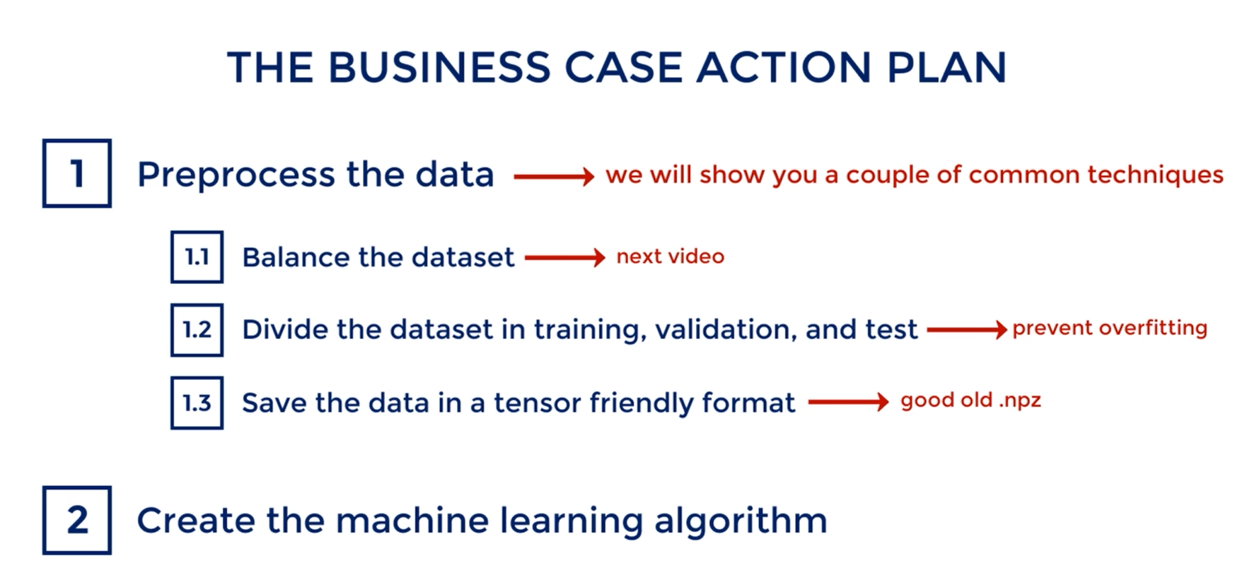
Balancing the dataset

We refer to the initial probability of picking a photo of some class as a prior.

A machine learning algorithm may quickly learn that one class is much more common than the other and decide all the ways to output the value with the higher prior.

That's the reason we have to balance the data.

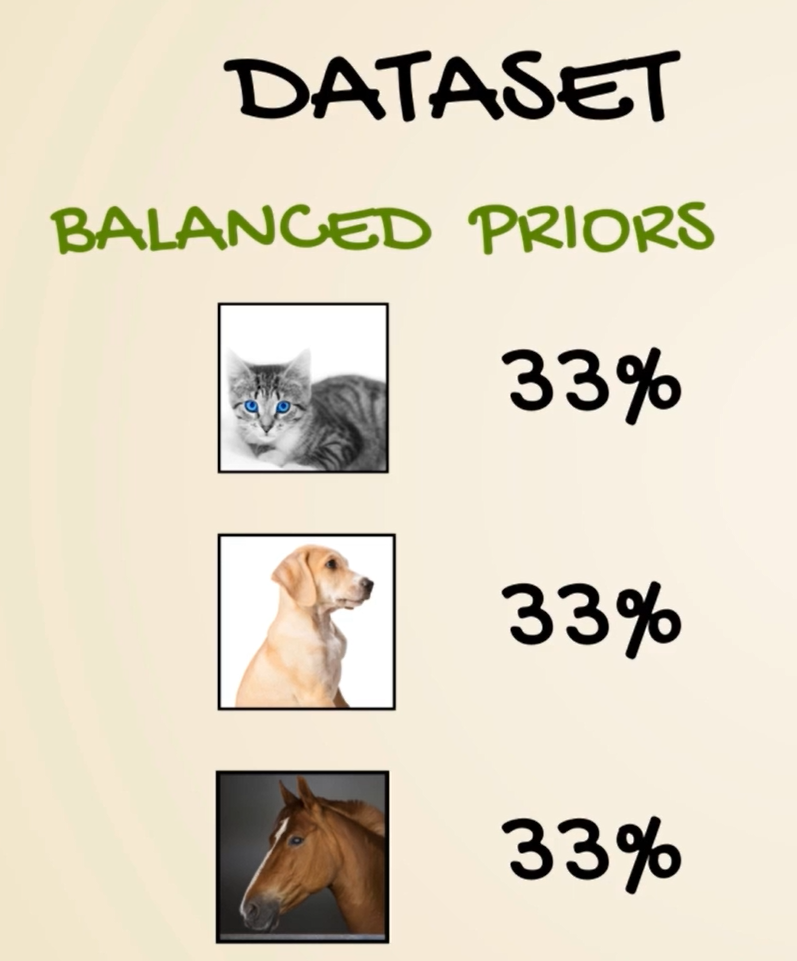
In our business case by exploring the targets we quickly realize most customers did not convert in the given time span.

We must surely balance the data set to proceed.

That's done by counting the total number of target ones and matching the same number of zeros to them.

Preprocessing the data

Extract the data from the csv:

First, let's import the libraries:

import numpy as np
from sklearn import preprocessing

We'll use the sklearn capabilities for standardizing the inputs.

It's one line of code which drastically improves the accuracy of the model, almost always we standardize all inputs as the quality of the algorithm improved significantly. Without standardizing the inputs we reach 10 percent less accuracy for the model.

First let's load the .csv file with a comma delimiter.

raw_csv_data = np.loadtxt('Audiobooks_data.csv', delimiter=',')

Now we have the data in a variable, our inputs are all the variables in the .csv except for the first and the last columns.

The first column is the arbitrarily chosen I.D. while the last is the targets.

Let's put that in a new variable, which takes all columns excluding the I.D. and the targets. So the 0 column and the last one or minus first.

unscaled_inputs_all = raw_csv_data[:, 1:-1]

Let's record the targets in the variable targets_all using the same method. They are the last column of the .csv.

Balance the dataset:

Now we'll deal with balancing the dataset.

1. We will count the number of targets that are 1, as we know they are less than the 0.

2. Next we will keep as many 0 as there are 1.

Let's count the targets that are 1. If we sum all targets which can take only 0 and 1 as value we will get the number of targets that are 1.

num_one_targets = int(np.sum(targets_all))

let's set a counter for the zero targets equal to zero.

Next we will need a variable that records the indices to be removed, for now it is empty, but we want it to be a list or a tuple, so we put empty brackets.

zeros_targets_counter = 0
indices_to_remove = []

Let's iterate over the dataset and balance it.

for i in range(targets_all.shape[0]):
    if targets_all[i]==0:
        zeros_targets_counter += 1
        if zeros_targets_counter > num_one_targets:
            indices_to_remove.append(i)

TIP

The shape of targets_all on axis = 0, is basically the length of the vector so it will show us the number of all targets.

In the loop, we want to increase the counter by 1 if the target at position i is 0. In that same if we put another if which will add an index to the variable indices_to_remove if the zeros_targets_counter is over the num_one_targets.

Then with the append method we simply add an element to the list.

So, after the counter for zeroes matches the number of ones I'll note all indices to be removed.

So, after we run the code the variable indices_to_remove will contain the indices of all targets we won't need. Deleting these entries will balance the data set.

Let's create a new variable:

unscaled_inputs_equal_priors = np.delete(unscaled_inputs_all, indices_to_remove, axis=0)

also,

targets_equal_priors = np.delete(targets_all, indices_to_remove, axis=0)

All right we have a balanced dataset.

Next, we want to standardize or scale the inputs.

Standardize the inputs:

The inputs are currently unscaled, and we noted that standardizing them will greatly improve the algorithm. A simple line of code takes care of that.

scaled_inputs = preprocessing.scale(unscaled_inputs_equal_priors)

That's the preprocessing library we imported from sklearn.

The scale method standardize is the data set along each variable.

So, basically, all inputs will be standardized.

So, we have a balanced dataset which is also scaled our preprocessing is almost finished.

Shuffeling the data:

A little trick is to shuffle the inputs and the targets. We are, basically, keeping the same information but in a different order.

It's possible that the original dataset was collected in the Order of Date since we will be batching, we must shuffle the data. It should be as randomly spread as possible so batching works fine.

First, we take the indices from the Axis 0 of these scaled inputs shape and place them into variable.

Then we use the np.random.shuffle() method to shuffle them.

shuffle_indices = np.arange(scaled_inputs.shape[0])
np.random.shuffle(shuffle_indices)

Finally, we create shuffled_inputs and shuffled_targets variables equal to the scaled inputs and the targets where the indices are the shuffle_indices.

shuffled_inputs = scaled_inputs[shuffle_indices]
shuffled_targets = targets_equal_priors[shuffle_indices]

So far, we have preprocessed the data, shuffled it, and balance the dataset.

What we have left is to split it into training, validation and test.

Split the dataset into train, validation, and test:

First, Let's count the total number of samples it is equal to the shape of the shuffled inputs on the 0 axis.

samples_count = shuffled_inputs.shape[0]

Next, We must determine the size of the three data sets.

I'll use the 80-10-10 split for train, validation, and test.

train_samples_count = int(0.8*samples_count)
validation_samples_count = int(0.1*samples_count)
test_samples_count = samples_count - train_samples_count - validation_samples_count

OK, we have the sizes of the train validation and test. Let's extract them from the big data set.

The train inputs are given by the first train samples count of the preprocessed inputs, the train targets are the first train samples count of the targets and, logically, the validation inputs are the inputs in the interval from train samples count to train samples counts + validation samples count, the validation targets are the targets in the same interval.

Finally, the test is everything that is left.

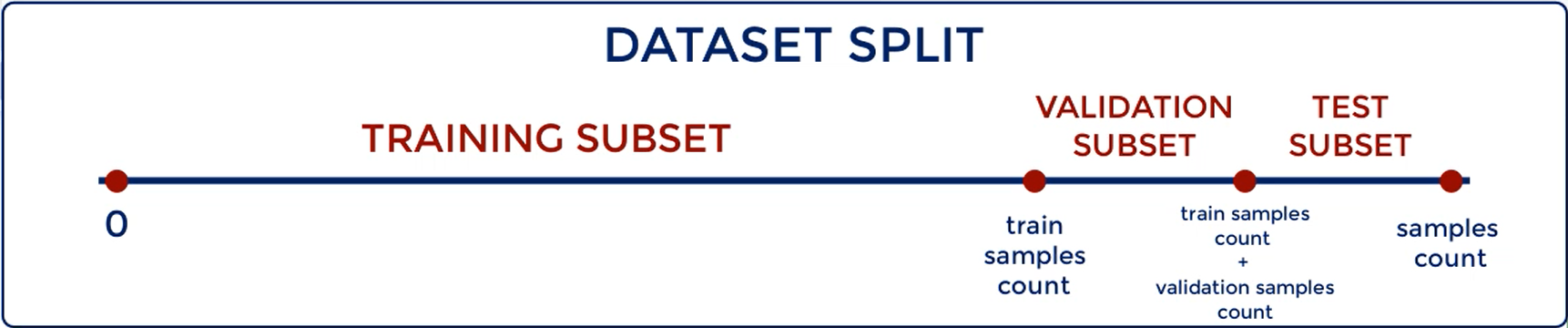
train_inputs = shuffled_inputs[:train_samples_count]
train_targets = shuffled_targets[:train_samples_count]

validation_inputs = shuffled_inputs[train_samples_count:train_samples_count+validation_samples_count]
validation_targets = shuffled_targets[train_samples_count:train_samples_count+validation_samples_count]

test_inputs = shuffled_inputs[train_samples_count+validation_samples_count:]
test_targets = shuffled_targets[train_samples_count+validation_samples_count:]

We have split the data set into training, validation and test

It is useful to check if we have balanced the dataset. Moreover, we may have balanced the whole dataset but not the training, validation and test sets

I'll print the number of 1 for each dataset, the total number of samples, and the proportion of 1 as a part of the total. They should all be around 50%.

1789.0 3579 0.49986029617211514
222.0 447 0.4966442953020134
226.0 448 0.5044642857142857

We can see the training set is considerably larger than the validation and the test. 3579 vs 447 and 448

This is how we wanted it to be. The total number of observations is around 4500 which is a relatively good amount of data, although, we started with around 15000 samples in the .csv.

The proportions, or should I say the Priors, look OK as they are almost 50%.

Note that 52% or 55% for two classes are also fine. However, we want to be as close to 50% as possible.

Finally, we save the three data sets using the np.savez() method. I name them in a very semantic way so we can easily use them later.

np.savez('Audiobooks_data_train', inputs=train_inputs, targets=train_targets)
np.savez('Audiobooks_data_validation', inputs=validation_inputs, targets=validation_targets)
np.savez('Audiobooks_data_test', inputs=test_inputs, targets=test_targets)

All right. Our data is pretty process now.

Each time we run the code, we will get different proportions, as we shuffle the indices randomly. So training, validation and test data sets will contain different samples.

You can use the same code to preprocess any data set where you have two classes.

The code will skip the first column of the data, as here we skip the I.D. and the last column will be treated as targets.

unscaled_inputs_all = raw_csv_data[:, 1:-1]
targets_all = raw_csv_data[:, -1]

If you want to customize the code for a problem with more classes, you must balance the data set classes instead of two, everything else should be the same.

The preprocessing is over. For now we will only work with the *.npz files.

Exercise: It makes sense to shuffle the indices prior to balancing the dataset.Using the code from the lesson, shuffle the indices and then balance the dataset. Note: This is more of a programming exercise rather than a machine learning one. Being able to complete it successfully will ensure you understand the preprocessing.

# When the data was collected it was actually arranged by date
# Shuffle the indices of the data, so the data is not arranged in any way when we feed it.
# Since we will be batching, we want the data to be as randomly spread out as possible
shuffled_indices = np.arange(unscaled_inputs_all.shape[0])
np.random.shuffle(shuffled_indices)

# Use the shuffled indices to shuffle the inputs and targets.
unscaled_inputs_all = unscaled_inputs_all[shuffled_indices]
targets_all = targets_all[shuffled_indices]

Loading the preprocessed data

Let's start by taking a look at the net we're going to deal with here.

We have an input layer consisting of 10 units. Those are the inputs from our .csv.

As you can see, there are only 2 output nodes, as there are only 2 possibilities 0 and 1. We will build a net with 2 hidden layers.

The number of units in each layer will be 50.

But, as we know very well, this is extremely easy to change. Therefore, for a prototype of an algorithm 50 is a good value.

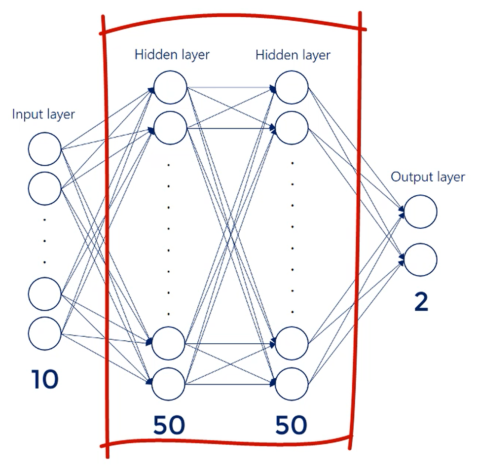
Let me explain in more detail, 50 hidden units in the hidden layers provide enough complexity. So we expect the algorithm to be much more sophisticated than a linear or logistic regression.

At the same time, we don't want to put too many units initially as we want to complete the learning as fast as possible, and see if anything is being learnd at all.

Create the Machine Learning Algorithm

First Let's import the libraries numpy and tensorflow.

import numpy as np
import tensorflow as tf

The next logical step is to load the data.

To make things easier, I'll declare a temporary variable called npz that will store each of the three data sets as we load, and to load the train data we use:

npz = np.load('Audiobooks_data_train.npz')

You probably remember that we saved the .npz in 2-tuple form comprising inputs and targets.

Let's start from the inputs and extract them into a new variable called train_inputs. Until now, they were stored in the .npz under the keyword inputs. So we call them as npz['inputs].

train_inputs = npz['inputs']

Finally, to make sure our model learns correctly we expect all inputs to be floats. Therefore, we must ensure that by employing the method astype()

train_inputs = npz['inputs'].astype(np.float)

In a similar way, we extract the train targets from .npz using the keyword targets.

Now, our targets are 0 and 1 but we are not completely certain if they'll be extracted as integers floats or booleans.

It's good practice to use the same method astype() and make sure their data type will be np.int even if we know in what format we save them.

train_targets = npz['targets'].astype(np.int)

All right we've got our train inputs and targets. What about the validation and test?

Well we start by loading the next .npz namely Audiobooks_data_validation in a temporary variable npz, then we proceed in a similar way to extract the validation inputs and targets, making sure of their data types.

npz = np.load('Audiobooks_data_validation.npz')

validation_inputs = npz['inputs'].astype(np.float)
validation_targets = npz['targets'].astype(np.int)

npz = np.load('Audiobooks_data_test.npz')

test_inputs = npz['inputs'].astype(np.float)
test_targets = npz['targets'].astype(np.int)

Finally, note that unlike before our train, validation and test data is simply an array form instead of the iterator we use for the MNIST.

In this business example, we will train our model with simple everyday arrays.

Learning and Interpret the Results

Throughout the entire course, we claim tenser flow code is extremely reusable. We will now prove this is in fact true.

Let me copy the MNIST model outline.

We're going to need a couple of adjustments though.

#%%
input_size = 784
output_size = 10
hidden_layer_size = 200

model = tf.keras.Sequential([
                            tf.keras.layers.Flatten(input_shape=(28, 28, 1)),
                            tf.keras.layers.Dense(hidden_layer_size, activation='relu'),
                            tf.keras.layers.Dense(hidden_layer_size, activation='relu'),
                            tf.keras.layers.Dense(output_size, activation='softmax'),
                            ])

First, the input size of our model must be 10 as there are 10 predictors.

Second, the output size of our model must be 2 as our targets are 0 or 1.

What about the hidden layer size?

We can leave it as it is because we aren't sure what the optimal value is.

input_size = 10
output_size = 2
hidden_layer_size = 200

Finally, in the amnesty code we use the method flatten to flatten each image into a vector.

This time though, we have already pre processed our data appropriately, so we can delete that line altogether. The rest remains unchanged.

model = tf.keras.Sequential([
                            tf.keras.layers.Dense(hidden_layer_size, activation='relu'),
                            tf.keras.layers.Dense(hidden_layer_size, activation='relu'),
                            tf.keras.layers.Dense(output_size, activation='softmax'),
                            ])

We've got 2 hidden layers, each activated by a relu activation function.

We know that our model is a classifier. Therefore, our output layer should be activated with SoftMax and that's all.

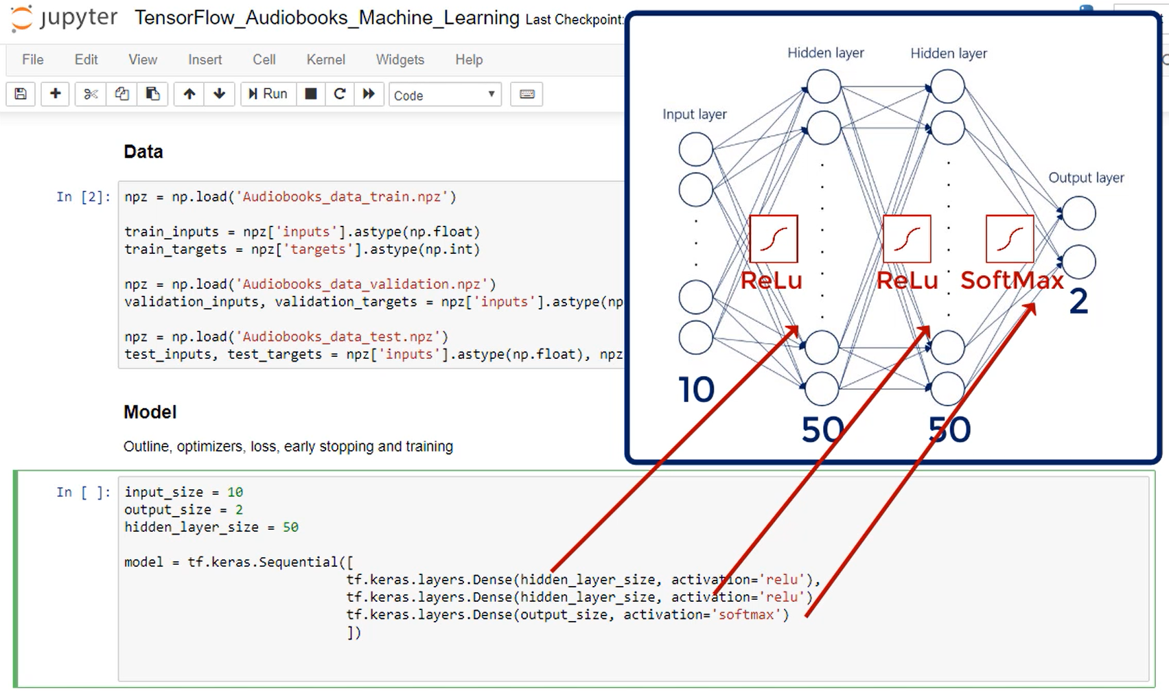
Next, we choose the optimizer and the loss function like before.

Let's copy paste that from the MNIST example.

model.compile(optimizer='adam', loss='sparse_categorical_crossentropy', metrics=['accuracy'])

The chosen optimizer is Adam. While the loss is sparse_categorical_crossentropy.

We use this loss to ensure that our integer targets are One-Hot encoded appropriately when calculating the loss.

Once again, we are happy with obtaining the accuracy for each batch.

We haven't set to have our hyper parameters yet the BATCH_SIZE and the max_epochs.

Speaking of batch size, we already said that, in this example, we won't take advantage of iterable objects that contain the data. Instead, we will employ simple arrays while the batching itself will be indicated when we fit the model in a minute or two.

All right, let's set both the batch size and the maximum number of epochs to 100.

batch_size = 100
max_epochs = 100

Next, we simply fit the model.

Let's start with the train inputs and the train targets.

We could feed a 2-tuple object containing both of them as we did with the MNIST, or we can feed them separately.

To show you both approaches, we already extracted the inputs and the targets into separate variables. OK, let's continue inside the fit method. We place the inputs first and then the targets.

model.fit(train_inputs, train_targets)

Next we've got the batch size.

If you were dealing with arrays as we are now, indicating the batch size here would automatically batch the data during the training process. So, batch_size=batch_size. What follows is the maximum number of epochs, epochs=max_epochs.

Regarding the validation data, There are two arrays of interest the validation inputs and the validation targets.

Finally, let's set verbose to 2.

model.fit(train_inputs,
          train_targets,
          batch_size=batch_size,
          epochs=max_epochs,
          validation_data=(validation_inputs, validation_targets,),
          verbose=2)

Let's run the code

Epoch 1/100
36/36 - 0s - loss: 0.4969 - accuracy: 0.7354 - val_loss: 0.4230 - val_accuracy: 0.7472
Epoch 2/100
36/36 - 0s - loss: 0.3864 - accuracy: 0.7921 - val_loss: 0.3896 - val_accuracy: 0.7875
Epoch 3/100
36/36 - 0s - loss: 0.3657 - accuracy: 0.8005 - val_loss: 0.3836 - val_accuracy: 0.7673
Epoch 4/100
36/36 - 0s - loss: 0.3558 - accuracy: 0.8100 - val_loss: 0.3925 - val_accuracy: 0.7494
Epoch 5/100
36/36 - 0s - loss: 0.3522 - accuracy: 0.8103 - val_loss: 0.3631 - val_accuracy: 0.7875
Epoch 6/100
36/36 - 0s - loss: 0.3442 - accuracy: 0.8153 - val_loss: 0.3568 - val_accuracy: 0.7852
Epoch 7/100
36/36 - 0s - loss: 0.3393 - accuracy: 0.8134 - val_loss: 0.3731 - val_accuracy: 0.7808
Epoch 8/100
36/36 - 0s - loss: 0.3378 - accuracy: 0.8173 - val_loss: 0.3657 - val_accuracy: 0.7808
Epoch 9/100
36/36 - 0s - loss: 0.3433 - accuracy: 0.8078 - val_loss: 0.3652 - val_accuracy: 0.7852
Epoch 10/100
36/36 - 0s - loss: 0.3282 - accuracy: 0.8248 - val_loss: 0.3541 - val_accuracy: 0.7875
Epoch 11/100
36/36 - 0s - loss: 0.3271 - accuracy: 0.8259 - val_loss: 0.3616 - val_accuracy: 0.8009
Epoch 12/100
36/36 - 0s - loss: 0.3293 - accuracy: 0.8195 - val_loss: 0.3920 - val_accuracy: 0.7875
Epoch 13/100
36/36 - 0s - loss: 0.3270 - accuracy: 0.8229 - val_loss: 0.3641 - val_accuracy: 0.7785
Epoch 14/100
36/36 - 0s - loss: 0.3297 - accuracy: 0.8108 - val_loss: 0.3709 - val_accuracy: 0.7740
Epoch 15/100
36/36 - 0s - loss: 0.3358 - accuracy: 0.8145 - val_loss: 0.3567 - val_accuracy: 0.7785
Epoch 16/100
36/36 - 0s - loss: 0.3204 - accuracy: 0.8262 - val_loss: 0.3505 - val_accuracy: 0.7875
Epoch 17/100
36/36 - 0s - loss: 0.3258 - accuracy: 0.8251 - val_loss: 0.3603 - val_accuracy: 0.7964
Epoch 18/100
36/36 - 0s - loss: 0.3243 - accuracy: 0.8223 - val_loss: 0.3628 - val_accuracy: 0.7964
Epoch 19/100
36/36 - 0s - loss: 0.3176 - accuracy: 0.8293 - val_loss: 0.3487 - val_accuracy: 0.7964
Epoch 20/100
36/36 - 0s - loss: 0.3176 - accuracy: 0.8270 - val_loss: 0.3460 - val_accuracy: 0.7808
Epoch 21/100
36/36 - 0s - loss: 0.3200 - accuracy: 0.8243 - val_loss: 0.3846 - val_accuracy: 0.7964
Epoch 22/100
36/36 - 0s - loss: 0.3275 - accuracy: 0.8203 - val_loss: 0.3602 - val_accuracy: 0.7919
Epoch 23/100
36/36 - 0s - loss: 0.3177 - accuracy: 0.8268 - val_loss: 0.3572 - val_accuracy: 0.8054
Epoch 24/100
36/36 - 0s - loss: 0.3238 - accuracy: 0.8195 - val_loss: 0.3691 - val_accuracy: 0.7897
Epoch 25/100
36/36 - 0s - loss: 0.3180 - accuracy: 0.8237 - val_loss: 0.3442 - val_accuracy: 0.8143
Epoch 26/100
36/36 - 0s - loss: 0.3147 - accuracy: 0.8321 - val_loss: 0.3498 - val_accuracy: 0.8076
Epoch 27/100
36/36 - 0s - loss: 0.3155 - accuracy: 0.8287 - val_loss: 0.3604 - val_accuracy: 0.8098
Epoch 28/100
36/36 - 0s - loss: 0.3181 - accuracy: 0.8231 - val_loss: 0.3664 - val_accuracy: 0.7763
Epoch 29/100
36/36 - 0s - loss: 0.3186 - accuracy: 0.8209 - val_loss: 0.3500 - val_accuracy: 0.7875
Epoch 30/100
36/36 - 0s - loss: 0.3139 - accuracy: 0.8296 - val_loss: 0.3490 - val_accuracy: 0.7763
Epoch 31/100
36/36 - 0s - loss: 0.3170 - accuracy: 0.8287 - val_loss: 0.3545 - val_accuracy: 0.8121
Epoch 32/100
36/36 - 0s - loss: 0.3237 - accuracy: 0.8203 - val_loss: 0.3621 - val_accuracy: 0.7987
Epoch 33/100
36/36 - 0s - loss: 0.3200 - accuracy: 0.8223 - val_loss: 0.3694 - val_accuracy: 0.7740
Epoch 34/100
36/36 - 0s - loss: 0.3119 - accuracy: 0.8310 - val_loss: 0.3603 - val_accuracy: 0.7919
Epoch 35/100
36/36 - 0s - loss: 0.3147 - accuracy: 0.8284 - val_loss: 0.4330 - val_accuracy: 0.7651
Epoch 36/100
36/36 - 0s - loss: 0.3179 - accuracy: 0.8290 - val_loss: 0.3699 - val_accuracy: 0.8009
Epoch 37/100
36/36 - 0s - loss: 0.3214 - accuracy: 0.8215 - val_loss: 0.3519 - val_accuracy: 0.7919
Epoch 38/100
36/36 - 0s - loss: 0.3131 - accuracy: 0.8329 - val_loss: 0.3587 - val_accuracy: 0.8054
Epoch 39/100
36/36 - 0s - loss: 0.3103 - accuracy: 0.8254 - val_loss: 0.3573 - val_accuracy: 0.7718
Epoch 40/100
36/36 - 0s - loss: 0.3129 - accuracy: 0.8284 - val_loss: 0.3534 - val_accuracy: 0.7785
Epoch 41/100
36/36 - 0s - loss: 0.3162 - accuracy: 0.8282 - val_loss: 0.4158 - val_accuracy: 0.7606
Epoch 42/100
36/36 - 0s - loss: 0.3204 - accuracy: 0.8170 - val_loss: 0.3565 - val_accuracy: 0.7919
Epoch 43/100
36/36 - 0s - loss: 0.3109 - accuracy: 0.8310 - val_loss: 0.3542 - val_accuracy: 0.7987
Epoch 44/100
36/36 - 0s - loss: 0.3108 - accuracy: 0.8259 - val_loss: 0.3640 - val_accuracy: 0.7852
Epoch 45/100
36/36 - 0s - loss: 0.3118 - accuracy: 0.8335 - val_loss: 0.3525 - val_accuracy: 0.8054
Epoch 46/100
36/36 - 0s - loss: 0.3114 - accuracy: 0.8298 - val_loss: 0.3478 - val_accuracy: 0.8031
Epoch 47/100
36/36 - 0s - loss: 0.3100 - accuracy: 0.8332 - val_loss: 0.3555 - val_accuracy: 0.7964
Epoch 48/100
36/36 - 0s - loss: 0.3125 - accuracy: 0.8237 - val_loss: 0.3858 - val_accuracy: 0.7852
Epoch 49/100
36/36 - 0s - loss: 0.3153 - accuracy: 0.8335 - val_loss: 0.3508 - val_accuracy: 0.7852
Epoch 50/100
36/36 - 0s - loss: 0.3110 - accuracy: 0.8312 - val_loss: 0.3467 - val_accuracy: 0.8098
Epoch 51/100
36/36 - 0s - loss: 0.3103 - accuracy: 0.8287 - val_loss: 0.3529 - val_accuracy: 0.8054
Epoch 52/100
36/36 - 0s - loss: 0.3101 - accuracy: 0.8296 - val_loss: 0.3498 - val_accuracy: 0.7964
Epoch 53/100
36/36 - 0s - loss: 0.3051 - accuracy: 0.8324 - val_loss: 0.3543 - val_accuracy: 0.7808
Epoch 54/100
36/36 - 0s - loss: 0.3042 - accuracy: 0.8349 - val_loss: 0.3516 - val_accuracy: 0.8076
Epoch 55/100
36/36 - 0s - loss: 0.3089 - accuracy: 0.8301 - val_loss: 0.3497 - val_accuracy: 0.7942
Epoch 56/100
36/36 - 0s - loss: 0.3079 - accuracy: 0.8326 - val_loss: 0.3682 - val_accuracy: 0.7830
Epoch 57/100
36/36 - 0s - loss: 0.3075 - accuracy: 0.8268 - val_loss: 0.3456 - val_accuracy: 0.8031
Epoch 58/100
36/36 - 0s - loss: 0.3103 - accuracy: 0.8298 - val_loss: 0.3670 - val_accuracy: 0.7919
Epoch 59/100
36/36 - 0s - loss: 0.3090 - accuracy: 0.8349 - val_loss: 0.3496 - val_accuracy: 0.8054
Epoch 60/100
36/36 - 0s - loss: 0.3099 - accuracy: 0.8324 - val_loss: 0.3509 - val_accuracy: 0.8121
Epoch 61/100
36/36 - 0s - loss: 0.3068 - accuracy: 0.8304 - val_loss: 0.3600 - val_accuracy: 0.8009
Epoch 62/100
36/36 - 0s - loss: 0.3058 - accuracy: 0.8324 - val_loss: 0.3497 - val_accuracy: 0.7808
Epoch 63/100
36/36 - 0s - loss: 0.3042 - accuracy: 0.8296 - val_loss: 0.3601 - val_accuracy: 0.7919
Epoch 64/100
36/36 - 0s - loss: 0.3154 - accuracy: 0.8326 - val_loss: 0.3818 - val_accuracy: 0.7740
Epoch 65/100
36/36 - 0s - loss: 0.3143 - accuracy: 0.8268 - val_loss: 0.3565 - val_accuracy: 0.7964
Epoch 66/100
36/36 - 0s - loss: 0.3075 - accuracy: 0.8365 - val_loss: 0.3535 - val_accuracy: 0.7785
Epoch 67/100
36/36 - 0s - loss: 0.3047 - accuracy: 0.8324 - val_loss: 0.3595 - val_accuracy: 0.7651
Epoch 68/100
36/36 - 0s - loss: 0.3076 - accuracy: 0.8245 - val_loss: 0.3487 - val_accuracy: 0.7964
Epoch 69/100
36/36 - 0s - loss: 0.3043 - accuracy: 0.8354 - val_loss: 0.3847 - val_accuracy: 0.7987
Epoch 70/100
36/36 - 0s - loss: 0.3107 - accuracy: 0.8324 - val_loss: 0.3562 - val_accuracy: 0.8166
Epoch 71/100
36/36 - 0s - loss: 0.3059 - accuracy: 0.8335 - val_loss: 0.3569 - val_accuracy: 0.7785
Epoch 72/100
36/36 - 0s - loss: 0.3046 - accuracy: 0.8301 - val_loss: 0.3512 - val_accuracy: 0.7964
Epoch 73/100
36/36 - 0s - loss: 0.3048 - accuracy: 0.8360 - val_loss: 0.3763 - val_accuracy: 0.7987
Epoch 74/100
36/36 - 0s - loss: 0.3045 - accuracy: 0.8371 - val_loss: 0.3736 - val_accuracy: 0.7897
Epoch 75/100
36/36 - 0s - loss: 0.3069 - accuracy: 0.8357 - val_loss: 0.3763 - val_accuracy: 0.7987
Epoch 76/100
36/36 - 0s - loss: 0.3071 - accuracy: 0.8265 - val_loss: 0.3781 - val_accuracy: 0.7808
Epoch 77/100
36/36 - 0s - loss: 0.3076 - accuracy: 0.8340 - val_loss: 0.3618 - val_accuracy: 0.7987
Epoch 78/100
36/36 - 0s - loss: 0.3044 - accuracy: 0.8393 - val_loss: 0.3487 - val_accuracy: 0.7875
Epoch 79/100
36/36 - 0s - loss: 0.3069 - accuracy: 0.8379 - val_loss: 0.3681 - val_accuracy: 0.7830
Epoch 80/100
36/36 - 0s - loss: 0.3064 - accuracy: 0.8273 - val_loss: 0.3596 - val_accuracy: 0.7606
Epoch 81/100
36/36 - 0s - loss: 0.3046 - accuracy: 0.8296 - val_loss: 0.3567 - val_accuracy: 0.7808
Epoch 82/100
36/36 - 0s - loss: 0.3060 - accuracy: 0.8321 - val_loss: 0.3853 - val_accuracy: 0.7942
Epoch 83/100
36/36 - 0s - loss: 0.3073 - accuracy: 0.8318 - val_loss: 0.3639 - val_accuracy: 0.7919
Epoch 84/100
36/36 - 0s - loss: 0.3068 - accuracy: 0.8321 - val_loss: 0.3567 - val_accuracy: 0.8076
Epoch 85/100
36/36 - 0s - loss: 0.3055 - accuracy: 0.8354 - val_loss: 0.3557 - val_accuracy: 0.7808
Epoch 86/100
36/36 - 0s - loss: 0.3019 - accuracy: 0.8304 - val_loss: 0.3610 - val_accuracy: 0.7852
Epoch 87/100
36/36 - 0s - loss: 0.3067 - accuracy: 0.8354 - val_loss: 0.3777 - val_accuracy: 0.7830
Epoch 88/100
36/36 - 0s - loss: 0.3030 - accuracy: 0.8329 - val_loss: 0.3844 - val_accuracy: 0.7919
Epoch 89/100
36/36 - 0s - loss: 0.3024 - accuracy: 0.8346 - val_loss: 0.3703 - val_accuracy: 0.7942
Epoch 90/100
36/36 - 0s - loss: 0.3028 - accuracy: 0.8343 - val_loss: 0.3655 - val_accuracy: 0.7852
Epoch 91/100
36/36 - 0s - loss: 0.3064 - accuracy: 0.8304 - val_loss: 0.3531 - val_accuracy: 0.8009
Epoch 92/100
36/36 - 0s - loss: 0.3073 - accuracy: 0.8256 - val_loss: 0.3544 - val_accuracy: 0.8009
Epoch 93/100
36/36 - 0s - loss: 0.3054 - accuracy: 0.8335 - val_loss: 0.3594 - val_accuracy: 0.7875
Epoch 94/100
36/36 - 0s - loss: 0.3010 - accuracy: 0.8335 - val_loss: 0.3553 - val_accuracy: 0.7897
Epoch 95/100
36/36 - 0s - loss: 0.2998 - accuracy: 0.8371 - val_loss: 0.3622 - val_accuracy: 0.7897
Epoch 96/100
36/36 - 0s - loss: 0.3028 - accuracy: 0.8284 - val_loss: 0.3549 - val_accuracy: 0.7852
Epoch 97/100
36/36 - 0s - loss: 0.3059 - accuracy: 0.8340 - val_loss: 0.3644 - val_accuracy: 0.7919
Epoch 98/100
36/36 - 0s - loss: 0.3060 - accuracy: 0.8368 - val_loss: 0.3680 - val_accuracy: 0.7897
Epoch 99/100
36/36 - 0s - loss: 0.3052 - accuracy: 0.8326 - val_loss: 0.3535 - val_accuracy: 0.7830
Epoch 100/100
36/36 - 0s - loss: 0.3057 - accuracy: 0.8354 - val_loss: 0.3562 - val_accuracy: 0.7964

Why did our model train for all 100 epochs isn't there a danger of over fitting after training for so long. Well, yes, precisely.

If we check the training process over time we'll notice that while the training loss was consistently decreasing our validation loss was sometimes increasing. So it's pretty obvious, we have overfitted when we train the MNIST.

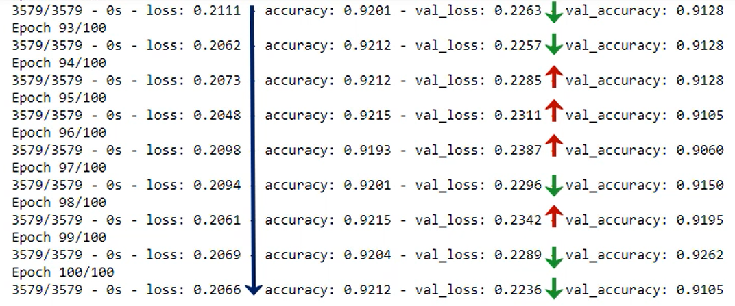
We didn't really set an early stopping procedure here.

Once again, we missed this step for the MNIST.

This was not really crucial. If you remember the dataset was so well pre process, that it would barely make a difference.

This time though, it does.

Setting an Early stopping mechanism

In this lecture, we'll explore how to set up an early stopping mechanism with tensor flow.

The fit method contains an argument called callbacks. Callbacks are functions called at certain points during model training.

Fortunately, there are many different readily available callbacks.

You can draw your training process and TensorBoard.

You can stream the results into a .csv file or a server.

Save the model after each epoch.

Adjust the learning rate in weird ways, and these are just some of the options.

You can also, define any custom callback you may want to use. However, the one we'll focus on is EarlyStopping.

And, no wonder, EarlyStopping is the definition of a utility called at a certain point during training.

Each time the validation loss is calculated, it is compared to the validation loss one epoch ago. If it starts increasing the model is overfitting and we should stop training.

Since the EarlyStopping mechanism is a hyper parameter, in a way, let's declare a new variable called early_stopping which will be an instance of tf.keras.callbacks.EarlyStopping.

As you can guess, there is a readily available structure we can use. So, all we need to take care of are the particulars of this early stopping mechanism.

By default, this object will monitor the validation loss and stop the training process the first time the validation loss starts increasing.

All right, now that we've got our early stopping mechanism, it's time to implement it in our training process.

model.fit(train_inputs,
          train_targets,
          batch_size=batch_size,
          epochs=max_epochs,
          callbacks=[early_stopping],
          validation_data=(validation_inputs, validation_targets),
          verbose=2)

Now, if we examine the validation loss, we'll notice that the first time it increased was during the last epoch. Moreover, it increased only slightly.

Sometimes, if we noticed that the validation loss has increased by an insignificant amount, we may prefer to let one or two validation increases slide to allow for this tolerance.

We can adjust the early stopping object. There is an argument called patience which by default is set to zero. There, we can specify the number of epochs with no improvement after which the training will be stopped.

It's a bit too strict to have no tolerance for a random increase in the validation loss. Therefore, let's set the patients to 2.

early_stopping = tf.keras.callbacks.EarlyStopping(patience=2)

The difference may not be crucial however this is yet another debugging tool of sorts that you have at your disposal.

Epoch 1/100
36/36 - 0s - loss: 0.5402 - accuracy: 0.7237 - val_loss: 0.4654 - val_accuracy: 0.7539
Epoch 2/100
36/36 - 0s - loss: 0.4537 - accuracy: 0.7698 - val_loss: 0.4286 - val_accuracy: 0.7629
Epoch 3/100
36/36 - 0s - loss: 0.4225 - accuracy: 0.7776 - val_loss: 0.4056 - val_accuracy: 0.7830
Epoch 4/100
36/36 - 0s - loss: 0.4020 - accuracy: 0.7916 - val_loss: 0.3950 - val_accuracy: 0.7852
Epoch 5/100
36/36 - 0s - loss: 0.3883 - accuracy: 0.7988 - val_loss: 0.3839 - val_accuracy: 0.7852
Epoch 6/100
36/36 - 0s - loss: 0.3799 - accuracy: 0.8036 - val_loss: 0.3855 - val_accuracy: 0.7808
Epoch 7/100
36/36 - 0s - loss: 0.3753 - accuracy: 0.8019 - val_loss: 0.3717 - val_accuracy: 0.7785
Epoch 8/100
36/36 - 0s - loss: 0.3688 - accuracy: 0.8089 - val_loss: 0.3677 - val_accuracy: 0.7785
Epoch 9/100
36/36 - 0s - loss: 0.3646 - accuracy: 0.8072 - val_loss: 0.3685 - val_accuracy: 0.7785
Epoch 10/100
36/36 - 0s - loss: 0.3608 - accuracy: 0.8075 - val_loss: 0.3554 - val_accuracy: 0.7875
Epoch 11/100
36/36 - 0s - loss: 0.3596 - accuracy: 0.8061 - val_loss: 0.3646 - val_accuracy: 0.7919
Epoch 12/100
36/36 - 0s - loss: 0.3600 - accuracy: 0.8041 - val_loss: 0.3547 - val_accuracy: 0.7852
Epoch 13/100
36/36 - 0s - loss: 0.3562 - accuracy: 0.8044 - val_loss: 0.3583 - val_accuracy: 0.7852
Epoch 14/100
36/36 - 0s - loss: 0.3544 - accuracy: 0.8061 - val_loss: 0.3551 - val_accuracy: 0.7875

Test the model

To test the model we use the method evaluate().

test_loss, test_accuracy = model.evaluate(test_inputs, test_targets)
print('\nTest Loss: {0:.2f}. Test accuracy: {1:.2f}%'.format(test_loss, test_accuracy*100.))

14/14 [==============================] - 0s 2ms/step - loss: 0.3313 - accuracy: 0.8438

Test Loss: 0.33. Test accuracy: 84.38%

From this point on I am no longer allowed to change the model.

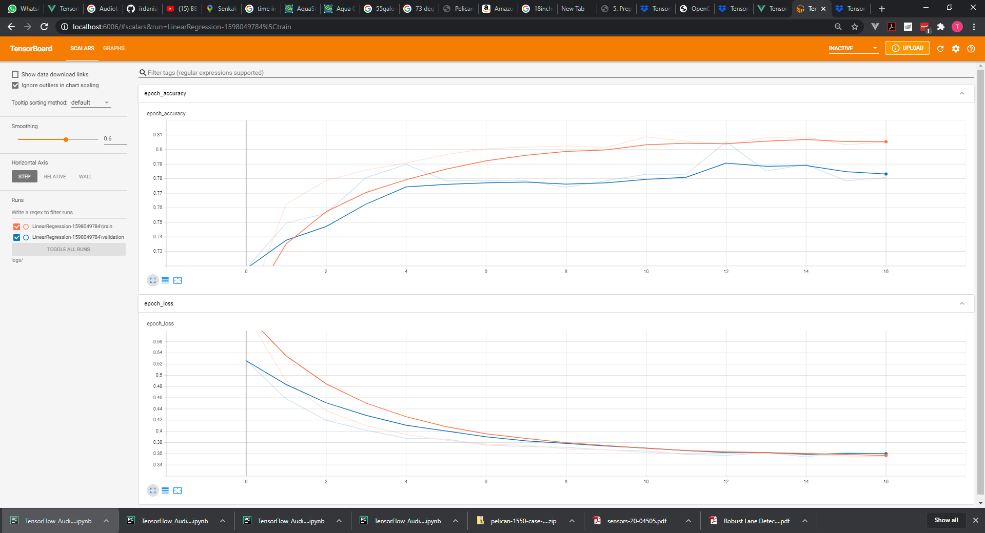
Preprocessing data

#%%
import numpy as np
from sklearn import preprocessing

raw_csv_data = np.loadtxt('Audiobooks_data.csv', delimiter=',')

unscaled_inputs_all = raw_csv_data[:, 1:-1]
targets_all = raw_csv_data[:, -1]

# When the data was collected it was actually arranged by date
# Shuffle the indices of the data, so the data is not arranged in any way when we feed it.
# Since we will be batching, we want the data to be as randomly spread out as possible
shuffled_indices = np.arange(unscaled_inputs_all.shape[0])
np.random.shuffle(shuffled_indices)

# Use the shuffled indices to shuffle the inputs and targets.
unscaled_inputs_all = unscaled_inputs_all[shuffled_indices]
targets_all = targets_all[shuffled_indices]

#%%
# Balance the dataset
num_one_targets = int(np.sum(targets_all))

zeros_targets_counter = 0

indices_to_remove = []

for i in range(targets_all.shape[0]):
    if targets_all[i]==0:
        zeros_targets_counter += 1
        if zeros_targets_counter > num_one_targets:
            indices_to_remove.append(i)

unscaled_inputs_equal_priors = np.delete(unscaled_inputs_all, indices_to_remove, axis=0)

targets_equal_priors = np.delete(targets_all, indices_to_remove, axis=0)

#%%
# Standardize the inputs
scaled_inputs = preprocessing.scale(unscaled_inputs_equal_priors)

#%%
# Shuffle the data

shuffle_indices = np.arange(scaled_inputs.shape[0])
np.random.shuffle(shuffle_indices)

shuffled_inputs = scaled_inputs[shuffle_indices]
shuffled_targets = targets_equal_priors[shuffle_indices]


#%%
# Split the dataset into train, validation, and test

samples_count = shuffled_inputs.shape[0]

train_samples_count = int(0.8*samples_count)
validation_samples_count = int(0.1*samples_count)
test_samples_count = samples_count - train_samples_count - validation_samples_count

train_inputs = shuffled_inputs[:train_samples_count]
train_targets = shuffled_targets[:train_samples_count]

validation_inputs = shuffled_inputs[train_samples_count:train_samples_count+validation_samples_count]
validation_targets = shuffled_targets[train_samples_count:train_samples_count+validation_samples_count]

test_inputs = shuffled_inputs[train_samples_count+validation_samples_count:]
test_targets = shuffled_targets[train_samples_count+validation_samples_count:]

print(np.sum(train_targets), train_samples_count, np.sum(train_targets)/train_samples_count)
print(np.sum(validation_targets), validation_samples_count, np.sum(validation_targets)/validation_samples_count)
print(np.sum(test_targets), test_samples_count, np.sum(test_targets)/test_samples_count)

#%%
# Save the three datasets in *.npz

np.savez('Audiobooks_data_train', inputs=train_inputs, targets=train_targets)
np.savez('Audiobooks_data_validation', inputs=validation_inputs, targets=validation_targets)
np.savez('Audiobooks_data_test', inputs=test_inputs, targets=test_targets)

Machine learning algorithm

#%%
import numpy as np
import tensorflow as tf
import time
from tensorflow.keras.callbacks import TensorBoard

NAME = "LinearRegression-{}".format(int(time.time()))
tensorboard = TensorBoard(log_dir='logs/{}'.format(NAME))

#%%
npz = np.load('Audiobooks_data_train.npz')

train_inputs = npz['inputs'].astype(np.float)
train_targets = npz['targets'].astype(np.int)

npz = np.load('Audiobooks_data_validation.npz')

validation_inputs = npz['inputs'].astype(np.float)
validation_targets = npz['targets'].astype(np.int)

npz = np.load('Audiobooks_data_test.npz')

test_inputs = npz['inputs'].astype(np.float)
test_targets = npz['targets'].astype(np.int)



#%%
input_size = 10
output_size = 2
hidden_layer_size = 50

model = tf.keras.Sequential([
                            tf.keras.layers.Dense(hidden_layer_size, activation='relu'),
                            tf.keras.layers.Dense(hidden_layer_size, activation='relu'),
                            tf.keras.layers.Dense(output_size, activation='softmax'),
                            ])

model.compile(optimizer='adam', loss='sparse_categorical_crossentropy', metrics=['accuracy'])


batch_size = 100
max_epochs = 100
early_stopping = tf.keras.callbacks.EarlyStopping(patience=2)

model.fit(train_inputs,
          train_targets,
          batch_size=batch_size,
          epochs=max_epochs,
          callbacks=[early_stopping, tensorboard],
          validation_data=(validation_inputs, validation_targets),
          verbose=2)


#%%
test_loss, test_accuracy = model.evaluate(test_inputs, test_targets)

#%%
print('\nTest Loss: {0:.2f}. Test accuracy: {1:.2f}%'.format(test_loss, test_accuracy*100.))