# Assessment 02: Computer Program

Thiago Lima Souto - Mat.: 19044686

Professor Dr. Frazer

Masters of Engineering - Mechatronics

Massey University - 2nd semester 2019 - Auckland

# Course Learning Outcomes Assessed:

Analyse a system and create a model and/or simulation.
Analyse an optimization task then find and apply an appropriate optimisation technique.
Work individually, or in groups, to achieve a solution.
Present the results of a simulation, modelling or optimisation task in an appropriate manner.
Tackle an open-ended task and return the best solution within a given time frame.

Weighting: 20% Due Date: 23/08/2019 This is an individual assessment.

In this assessment you are required to create a formulation for the following optimisation problem and optimise its objective function:

FastPCB Ltd is a local Printed Circuit Board (PCB) manufacturer. Currently, employees transfer PCBs from one machine to another by hand. FastPCB has asked Massey University to develop a mobile robot to assist in PCB transportation. The company has provided the following map of the factory and desired waypoints for the robot:

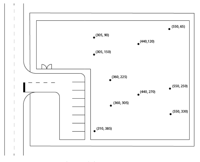
You need to decide on the path the robot will travel along, so that it minimizes the total distance travelled while visiting each waypoint once. It is planned for the robot to be stored at waypoint (310, 385).

Aims

Practice problem formulation and optimisation.

Objectives

Create a formulation for the optimisation problem.
Write a program to optimise the formulation’s objective function.

Requirements

Write a program that achieves the assessment’s objectives.
Write a short report detailing what you did, how, and why.

Submission Instructions

Add all your work to a .zip archive and name it in the following format: FIRSTNAME_LASTNAME_ID.zip. Be sure to include your program’s source code. Upload your submission to Stream before the due date. A 5 % per day penalty will be applied to late submissions.

# Solution

# The optimisation task

The proposed problem can be classified as one of the most known problems of computer science, the traveling salesman problem.

This problem was first mathematically formulated in the 1800s by W.R. Hamilton and Thomas Kirkman, although the general form seems to be first studied in 1930 by Karl Menger, he defines the problem, consider obvious brute-force algorithms and observes the non-optimality of the nearest neighbour heuristic, in which the rule that one first should go from the starting point to the nearest one and so on in general does not yield to the shortest route.

Since then, this problem has been studied by many mathematicians, computer scientists and with the advance of technology and modern ways of solving mathematical problems It is quite an easy task with many tools to solve. In the next topic this report will discuss these tools and how the problem can be solved.

# How to solve the problem

One of the ways to solve this problem is by brute-force, since It has only 10 nodes. This can be tried by trying all the permutations and compare to find the "cheapest" ways, although with this approach the the running time would be of $O(n!)$ and would be impractical for small amount of locations, such as 20. And this also would include the calculation of the distance between each point, which be can calculated by $\sqrt[]{(x2-x1)^2 + (y2-y1)^2}$ . This can be minimized by using some of the earliest application of dynamic programming like the Held-Karp algorithm which solve the problem in time $O(n^2 2^n)$ but still a very difficult way of solving the problem.

Some other techniques can increasingly solve this problem for quite a numerous amount of locations as shown on the table below:

Technique	Number of locations
branch-and-bound algorithms	40–60
Progressive improvement algorithms	up to 200 locations.
branch-and-cut algorithms	85,900 locations
Heuristic and approximation algorithms	millions of locations, with probability 2–3% away from the optimal solution.

Using modern computational libraries like OR-tools from google, programs like Matlab from Mathworks, Scipy or even Javascript libraries can handle this problem in a fairly simple way. The library we choose (OR-tools from google) will use an heuristic algorithm for example.

# Variables, Constraints and Objective function

# Variables

The variables of the problem will be all the locations, in more sophisticated problems these locations will be changing with time and a new best route has to be generated based on the new variables.

# Constraints

The constraints are basically that you have to come back to origin point, not repeat any node and choose the fastest way to complete the task.

# Objective function

The objective function in our case will use the parameters defined by the OR-Tools library with a first solution approach and the cheapest route. Where the algorithm will start the analysis from a starting point and look for the cheapest route.

search_parameters.first_solution_strategy = (routing_enums_pb2.FirstSolutionStrategy.PATH_CHEAPEST_ARC)

# The Graph analysis

A Graph is normally used to solve this kind of problem.

By Analyzing the possibilities we can start building a Graph with all possible routes, although, as we can see on the graphic below, after the second node the complexity increases.

For better visualization we can exclude the arrows and consider each way a two way via, and then we have the following Graph for the proposed problem.

# Tools and ways used to solve the problem

# Python + Visual Studio + OR-Tools

OR-Tools is a Google developed library specialized in optimization problems. For the proposed problem we are going to be using the vehicle routing library, a group of algorithms designed especially for the traveling salesman problem. this tools is optimal also for the amount of resources available. As mentioned before other tools could be used as well.

Visual Studio among many other programming languages can be used to do this task, like PyCharm or any other programming language IDE. Visual Studio was chosen because of the tool that simulates the Jupyter server on the fly, making them a simpler pipeline to achieve the results.

Python was chosen because of the flexibility of the language that is now used in many different fields like machine learning, AI, Data Science, robotics as well as web development and many others. Python can also use the benefits of C by using the Cyton approach.

Other aspect that was considered in the tools selection was the fact that Python OR-Tools and Visual Studio are free tools.

# The problem solution implementation

Importing the libraries necessary to perform the task, two common math and print and two solvers routing_enum_pb2 and pywarpcp:

from __future__ import print_function
import math
from ortools.constraint_solver import routing_enums_pb2
from ortools.constraint_solver import pywrapcp

1
2
3
4

Creating the Data model with the location of the waypoints for the robot, the number of robots and the starting point. In this case starting at 0.

def create_data_model():
    """Stores the data for the problem."""
    data = {}
    # Locations in block units
    data['locations'] = [     
        (310, 385), (305, 90), (305, 150), (360, 225), (360, 305),
        (440, 120), (440, 270), (550, 65), (550, 250), (550, 330),  
    ]  # yapf: disable
    data['num_vehicles'] = 1
    data['depot'] = 0
    return data

1
2
3
4
5
6
7
8
9
10
11

With the data setup we now have to calculate the Euclidean distance matrix.

As mentioned before this will be calculated with the distance between 2 points: $\sqrt[]{(x2-x1)^2 + (y2-y1)^2}$ , which in this case is the function math.hypot.


def compute_euclidean_distance_matrix(locations):
    """Creates callback to return distance between points."""
    distances = {}
    for from_counter, from_node in enumerate(locations):
        distances[from_counter] = {}
        for to_counter, to_node in enumerate(locations):
            if from_counter == to_counter:
                distances[from_counter][to_counter] = 0
            else:
                # Euclidean distance
                distances[from_counter][to_counter] = (int(
                    math.hypot((from_node[0] - to_node[0]),
                               (from_node[1] - to_node[1]))))
    return distances

1
2
3
4
5
6
7
8
9
10
11
12
13
14
15

This function will return all the distance between every point related to each other as shown below:

{
0: {0: 0, 1: 295, 2: 235, 3: 167, 4: 94, 5: 295, 6: 173, 7: 400, 8: 275, 9: 246},
1: {0: 295, 1: 0, 2: 60, 3: 145, 4: 221, 5: 138, 6: 225, 7: 246, 8: 292, 9: 342},
2: {0: 235, 1: 60, 2: 0, 3: 93, 4: 164, 5: 138, 6: 180, 7: 259, 8: 264, 9: 304},
3: {0: 167, 1: 145, 2: 93, 3: 0, 4: 80, 5: 132, 6: 91, 7: 248, 8: 191, 9: 217},
4: {0: 94, 1: 221, 2: 164, 3: 80, 4: 0, 5: 201, 6: 87, 7: 306, 8: 197, 9: 191}, 
5: {0: 295, 1: 138, 2: 138, 3: 132, 4: 201, 5: 0, 6: 150, 7: 122, 8: 170, 9: 237}, 
6: {0: 173, 1: 225, 2: 180, 3: 91, 4: 87, 5: 150, 6: 0, 7: 232, 8: 111, 9: 125}, 
7: {0: 400, 1: 246, 2: 259, 3: 248, 4: 306, 5: 122, 6: 232, 7: 0, 8: 185, 9: 265}, 
8: {0: 275, 1: 292, 2: 264, 3: 191, 4: 197, 5: 170, 6: 111, 7: 185, 8: 0, 9: 80}, 
9: {0: 246, 1: 342, 2: 304, 3: 217, 4: 191, 5: 237, 6: 125, 7: 265, 8: 80, 9: 0}
}

1
2
3
4
5
6
7
8
9
10
11
12
13

Analyzing the origin and the cost of all possible ways to the other locations we can start a graph like shown below. The compute_euclidean_distance_matrix function did these same calculations for all other locations.

Cost from Start location

Next step is to define how to print the solution. In this case basically we are printing the location + -> and next location.


def print_solution(manager, routing, assignment):
    """Prints assignment on console."""
    print('Objective: {}'.format(assignment.ObjectiveValue()))
    index = routing.Start(0)
    plan_output = 'Route:\n'
    route_distance = 0
    while not routing.IsEnd(index):
        plan_output += ' {} ->'.format(manager.IndexToNode(index))
        previous_index = index
        index = assignment.Value(routing.NextVar(index))
        route_distance += routing.GetArcCostForVehicle(previous_index, index, 0)
    plan_output += ' {}\n'.format(manager.IndexToNode(index))
    print(plan_output)
    plan_output += 'Objective: {}m\n'.format(route_distance)

1
2
3
4
5
6
7
8
9
10
11
12
13
14
15
16

Now that everything is setup we can analyse the main function.

On the main function we have to first call the "create_data_model" function and create a "data" variable to receive the data.

To create the Routing Model we use the pywrapcp library and pass the Locations, number of vehicles and depart location to the RoutingIndexManager function. After that we can create a variable and store the Euclidean Matrix by calling the "compute_euclidean_distance_matrix" function early defined.

A function has to be defined to return the distance between the nodes, as well as to define the cost of each arc.

This library will solve the problem using a Heuristic approach, mentioned early on the report, and after all we solve the problem using the "routing.SolveWithParameters" and print the answer.

The "first solution strategy" will be the on of choice. This solution strategy is the method the solver uses to find an initial solution.

Within the option for this method "PATH_CHEAPEST_ARC" starts from a route starting node and connects it to the node that produces the cheapest route segment, then It extend the route by iterating on the last node added to the route.

A similar option would be the "EVALUATOR_STRATEGY" which differs by analyzing the cost based on a function $SetFirstSolutionEvaluator()$ .

In this case we are using the "PATH_CHEAPEST_ARC" because we have defined the cost with the distance callback function.

def main():
    """Entry point of the program."""
    # Instantiate the data problem.
    data = create_data_model()

    # Create the routing index manager.
    manager = pywrapcp.RoutingIndexManager(
        len(data['locations']), data['num_vehicles'], data['depot'])

    # Create Routing Model.
    routing = pywrapcp.RoutingModel(manager)

    distance_matrix = compute_euclidean_distance_matrix(data['locations'])

    def distance_callback(from_index, to_index):
        """Returns the distance between the two nodes."""
        # Convert from routing variable Index to distance matrix NodeIndex.
        from_node = manager.IndexToNode(from_index)
        to_node = manager.IndexToNode(to_index)
        return distance_matrix[from_node][to_node]

    transit_callback_index = routing.RegisterTransitCallback(distance_callback)

    # Define cost of each arc.
    routing.SetArcCostEvaluatorOfAllVehicles(transit_callback_index)

    # Setting first solution heuristic.
    search_parameters = pywrapcp.DefaultRoutingSearchParameters()
    search_parameters.first_solution_strategy = (
        routing_enums_pb2.FirstSolutionStrategy.PATH_CHEAPEST_ARC)

    # Solve the problem.
    assignment = routing.SolveWithParameters(search_parameters)

    # Print solution on console.
    if assignment:
        print_solution(manager, routing, assignment)

if __name__ == '__main__':
    main()

1
2
3
4
5
6
7
8
9
10
11
12
13
14
15
16
17
18
19
20
21
22
23
24
25
26
27
28
29
30
31
32
33
34
35
36
37
38
39
40

# The Output

Jupyter Server URI: http://localhost:8888/?token=e0e7d66841f3d8d5b3e8c6b453630b398380817ef6c2df55
Python version:
3.7.3 (default, Mar 27 2019, 17:13:21) [MSC v.1915 64 bit (AMD64)]
(5, 7, 8)
C:\\ProgramData\\Anaconda3\\python.exe

from __future__ import print_function...
Objective: 1150
Route:
 0 -> 4 -> 3 -> 2 -> 1 -> 5 -> 7 -> 8 -> 9 -> 6 -> 0

1
2
3
4
5
6
7
8
9
10

On the original Graph formulated we can identify the optimized path between the numerous possible routes as shown below.

Finally, a graphical solution for the problem is presented: