Assessment 01 - Multiperiod linear program

Thiago Lima Souto - Mat.: 19044686

Professor Dr. Frazer

Masters of Engineering - Mechatronics

Massey University - 2nd semester 2019 - Auckland

Course: 282.758 – Simulation, Modelling and Optimisation Assessment: Assessment 01 – Written Assignment. Course Learning Outcomes Assessed:

• Analyse a system and create a model and/or simulation.
• Analyse an optimisation task then find and apply an appropriate optimisation technique.
• Work individually, or in groups, to achieve a solution.

Weighting: 10%. Due Date: 02/08/2019. This is an individual assessment.

Home

• Introduction
• Aims
• Objectives
• Requirements
• Submission Instructions
• Formulating the problem as a LP.
• Paper problem formulation
• Optimising the LP’s objective function
  • Python and Google OR-tools solution.
  • Solving as a Integer Program
• Chemical X sent to recycling

Introduction

In this assessment, you are required to formulate the following optimisation problem as a Linear Program (LP) and optimise its objective function:

The CRUD chemical plant produces as part of its production process a noxious compound called Chemical X. Chemical X is highly toxic and needs to be disposed of properly. Fortunately, CRUD is linked by a pipe system to the FRESHAIR recycling plant, which can safely re-process chemical X. On any given day, the CRUD plant will produce the following amount of Chemical X (the plant operates between 9 A.M. and 3 P.M. only):

Time	9 – 10 A.M.	10 – 11 A.M.	11 A.M. – 12 P.M.	12 – 1 P.M.	1–2 P.M.	2–3 P.M.
Chemical X (L)	300	240	600	200	300	900

Because of environmental regulations, at no point in time is the CRUD plant allowed to keep more than 1000 litres on site and no Chemical X can be kept overnight. At the top of every hour, an arbitrary amount of Chemical X can be sent to the FRESHAIR recycling plant. The cost of recycling Chemical X is different for every hour:

Time	10 A.M.	11 A.M.	12 P.M.	1 P.M.	2 P.M.	3 P.M.
Price ($ per L)	30	40	35	45	38	50

You need to decide on how much Chemical X to send from the CRUD plant to the FRESHAIR recycling plant at the top of each hour, so that you can minimise the total recycling cost, but also meet all the environmental constraints.

Aims

The assessment’s aims are to:

• Practice problem formulation and optimisation.

Objectives

The assessment’s objectives are to:

• Formulate the problem as a LP.
• Optimise the LP’s objective function.

Requirements

You are required to:

• Complete the assessment’s objectives.
• Write a short report detailing what you did, how, and why.

Submission Instructions

Add all your work to a .zip archive and name it in the following format: FIRSTNAME_LASTNAME_ID.zip. Be sure to include any source code, programs, notes, etc. Upload your submission to Stream before the due date.

Resolution Assessment 01:

Formulating the problem as a LP.

Defining the variables:

$xi$ = Amount recycled at $i$ o'clock, for $i = (10 - 15)$

$pi$ = Amount kept in the plant at $i$ o'clock, for $i = (10 - 14)$

Obs.: $p9$ and $p15 = 0$

Objective function: How much Chemical X to send from the CRUD plant to the FRESHAIR recycling plant at the top of each hour, so that you can minimize the total recycling cost. This cost is the amount charged on a particular hour times the amount sent for recycling on that hour, as expressed bellow:

$30x10 + 40x11 + 35x12 + 45x13 + 38x14 + 50x15$

Constraints:

• No Chemical X can be kept overnight;

• At no point in time is the CRUD plant allowed to keep more than 1000 litres on site.

TIP

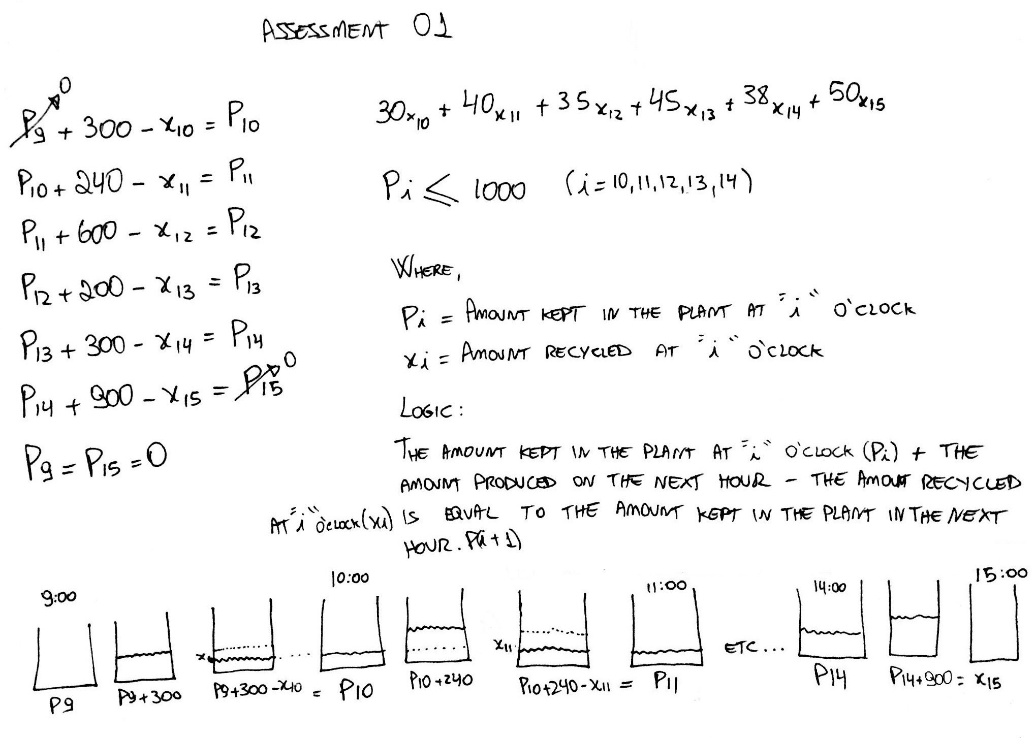
Logic: The amount kept in the plant at $i$ o'clock ($p_i$) + the amount produced on the next hour - the amount recycled at $i$ o'clock is equal to the amount kept in the plant in the next hour ($p_{i+1}$).

1. $300 - x10 = p10$

2. $p10 + 240 - x11 = p11$

3. $p11 + 600 - x12 = p12$

4. $p12 + 200 - x13 = p13$

5. $p13 + 300 - x14 = p14$

6. $p14 + 900 - x15 = 0$

Paper problem formulation

Optimising the LP’s objective function

Python and Google OR-tools solution.

To optimise the objective function a Python program was used importing the "Solver" tool imported from the "pywraplp" library of the Google OR-Tools tools package.

To find a formulation for the problem the following steps were taken:

1. Eleven variables were defined
2. A objective function was determined
3. Six constraints were determined

The command solver.Minimize was applied on the objective function and the values of $xi(i = 10-15)$ were printed on the terminal window as reported below:

from ortools.linear_solver import pywraplp

def main():
    'main'

    solver = pywraplp.Solver('mixed_integer_multiperiod', pywraplp.Solver.CBC_MIXED_INTEGER_PROGRAMMING)

    infinity = solver.infinity()

    x10 = solver.IntVar(0, infinity, 'x10')
    x11 = solver.IntVar(0, infinity, 'x11')
    x12 = solver.IntVar(0, infinity, 'x12')
    x13 = solver.IntVar(0, infinity, 'x13')
    x14 = solver.IntVar(0, infinity, 'x14')
    x15 = solver.IntVar(0, infinity, 'x15')
    p10 = solver.IntVar(0, 1000, 'p10')
    p11 = solver.IntVar(0, 1000, 'p11')
    p12 = solver.IntVar(0, 1000, 'p12')
    p13 = solver.IntVar(0, 1000, 'p13')
    p14 = solver.IntVar(0, 1000, 'p14')

    print('Number of Variables = ', solver.NumVariables())

    solver.Add(300-x10 == p10)
    solver.Add(p10 + 240 - x11 == p11)
    solver.Add(p11 + 600 - x12 == p12)
    solver.Add(p12 + 200 - x13 == p13)
    solver.Add(p13 + 300 - x14 == p14)
    solver.Add(p14 + 900 - x15 == 0)

    print('Number of Constraints = ', solver.NumConstraints())

    solver.Minimize(30*x10 + 40*x11 + 35*x12 + 45*x13 + 38*x14 + 50*x15)

    results_status = solver.Solve()

    assert results_status == pywraplp.Solver.OPTIMAL

    assert solver.VerifySolution(1e-7, True)

    print('Solution:')
    print('Objective value =', solver.Objective().Value())
    print('x10 = ', x10.solution_value())
    print('x11 = ', x11.solution_value())
    print('x12 = ', x12.solution_value())
    print('x13 = ', x13.solution_value())
    print('x14 = ', x14.solution_value())
    print('x15 = ', x15.solution_value())

    print('\nAdvanced usage:')
    print('Problem solved in %f milliseconds' % solver.wall_time())
    print('Problem solved in %d iterations' % solver.iterations())
    print('Problem solved in %d branch-and-bound nodes' % solver.nodes())

if __name__ == '__main__':
    main()

Console Result

Number of Variables =  11
Number of Constraints =  6
Solution:
Objective value = 102400.0
x10 =  300.0
x11 =  0.0
x12 =  840.0
x13 =  0.0
x14 =  500.0
x15 =  900.0

Advanced usage:
Problem solved in 2.000000 milliseconds
Problem solved in 0 iterations
Problem solved in 0 branch-and-bound nodes

Solving as a Integer Program

For that we have to change the solver to "pywraplp.Solver.CBC_MIXED_INTEGER_PROGRAMMING" and also cahnge the variables from NumVar to IntVar, as shown below.

from ortools.linear_solver import pywraplp

def main():
    'main'

    solver = pywraplp.Solver('mixed_integer_multiperiod', pywraplp.Solver.CBC_MIXED_INTEGER_PROGRAMMING)

    infinity = solver.infinity()

    x10 = solver.IntVar(0, infinity, 'x10')
    x11 = solver.IntVar(0, infinity, 'x11')
    x12 = solver.IntVar(0, infinity, 'x12')
    x13 = solver.IntVar(0, infinity, 'x13')
    x14 = solver.IntVar(0, infinity, 'x14')
    x15 = solver.IntVar(0, infinity, 'x15')
    p10 = solver.IntVar(0, 1000, 'p10')
    p11 = solver.IntVar(0, 1000, 'p11')
    p12 = solver.IntVar(0, 1000, 'p12')
    p13 = solver.IntVar(0, 1000, 'p13')
    p14 = solver.IntVar(0, 1000, 'p14')

    print('Number of Variables = ', solver.NumVariables())

    solver.Add(300-x10 == p10)
    solver.Add(p10 + 240 - x11 == p11)
    solver.Add(p11 + 600 - x12 == p12)
    solver.Add(p12 + 200 - x13 == p13)
    solver.Add(p13 + 300 - x14 == p14)
    solver.Add(p14 + 900 - x15 == 0)

    print('Number of Constraints = ', solver.NumConstraints())

    solver.Minimize(30*x10 + 40*x11 + 35*x12 + 45*x13 + 38*x14 + 50*x15)

    results_status = solver.Solve()

    assert results_status == pywraplp.Solver.OPTIMAL

    assert solver.VerifySolution(1e-7, True)

    print('Solution:')
    print('Objective value =', solver.Objective().Value())
    print('x10 = ', x10.solution_value())
    print('x11 = ', x11.solution_value())
    print('x12 = ', x12.solution_value())
    print('x13 = ', x13.solution_value())
    print('x14 = ', x14.solution_value())
    print('x15 = ', x15.solution_value())

    print('\nAdvanced usage:')
    print('Problem solved in %f milliseconds' % solver.wall_time())
    print('Problem solved in %d iterations' % solver.iterations())
    print('Problem solved in %d branch-and-bound nodes' % solver.nodes())

if __name__ == '__main__':
    main()

The results will be the same for this example:

Number of Variables =  11
Number of Constraints =  6
Solution:
Objective value = 102400.0
x10 =  300.0
x11 =  0.0
x12 =  840.0
x13 =  0.0
x14 =  500.0
x15 =  900.0

Advanced usage:
Problem solved in 2.000000 milliseconds
Problem solved in 0 iterations
Problem solved in 0 branch-and-bound nodes

Chemical X sent to recycling

Graphical Analysis:

By analyzing the graph we can tell that biggest amount of Chemical X were sent at 12 and 3 P.M., at 10 A.M. everything that could have been sent was sent because of the cheapest price and at the most expensive hour the plant had no other choice than to send everything that was produced, 900 litres. Although no Chemical X was sent at 11 A.M and 1 P.M., because of the price. The minimum cost of recycling was achieved at $102.400,00.