INTRODUCTION

Industrial robot systems as well as computer-aided design and manufacturing (CAD and CAM) are leading the industrial automation. [1]

The mechanical manipulator is the most important form of the industrial robot and the localization of objects in the three-dimensional space is one of the most important aspect of the mechanical manipulator. Links, parts, tools, other objects on the manipulator environment and the motion of these objects are the subjects of study of Kinematics, as well as all the geometrical and time-based properties of the motion, with no regards to the forces applied that causes it.

The two basic problems in the study of mechanical manipulation are forward and inverse kinematics, the first computes the position and orientation of the end-effector on the manipulator and the second calculates all possible sets of joint angles that could be used a given position and orientation.

Nowadays, CAD and CAM advanced software's are of easy access and used to design, simulate and calculate all that is necessary for modern robot design.

The main objective of this assessment is to design a robotic manipulator with a fixed platform and flat surface, that is able to be integrated with a robot gripper for picking an object vertical wall/shelf and placing it onto a horizontal surface.

To accomplish this objective a robot system is proposed after this introduction followed by the manipulator and other components design. The forward and inverse kinematics of the robot system are studied with manual calculations as well as computed calculations. A Model with correct dimensions and a simulation of the proposed robot are made using Solidworks and OpenModelica.

Finally, the results are discussed and the report is concluded.

Robot System Initial Proposal

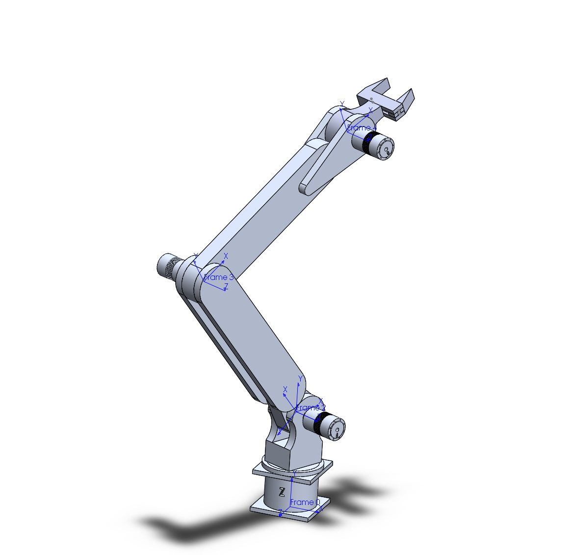
Aiming on the objective of designing a robot system, basically, capable of picking an object from a shelf and placing it onto a horizontal surface, the system proposed is a 4$dof$ (degrees of freedom, calculated using Grubler's formula) robot manipulator, consisting of a fixed base, a rotating base, two solid links and a toll, as shown in the Figure below.

$\begin{matrix} dof = m(N-1-J) + \sum_{i=1}^{J} f_i \\ dof = 6(5-1-4) + 4 \\ dof = 4 \end{matrix} \qquad(1)$

Where,

$N$ = number of bodies, counting ground as one body.

$J$ = Number of joints.

$m$ = 6 for spatial bodies.

$f_i$ = degrees of freedom of each joint. \end{eqfloat} To control the joints four brushless AC motors are used. The motors have attached a magnetic absolute encoder and a integrated controller. At the end of the system there is a simple gripper making the robotic manipulator able to pickup an object and place it onto a horizontal surface.

Manipulator Design

Robot Arms

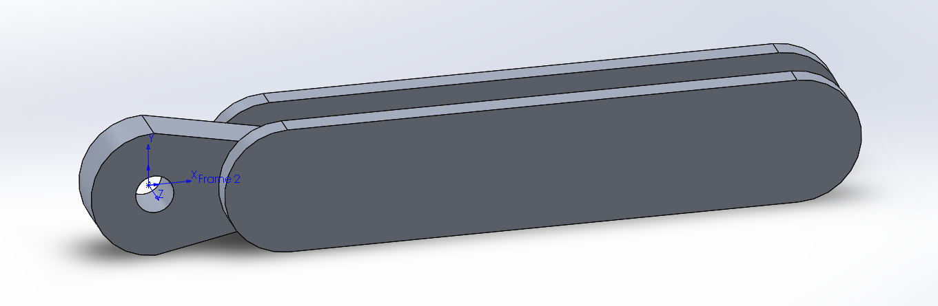
Link 1 and Link 2 constitute the "arms" of the manipulator, they are designed to maximize the joint angle reach for more flexibility. Also in the rotation base there are two cuts two maximize even further the arms reach as can be seen on Figure below. In this picture, with the Wireframe view with hidden lines visible, the fourth motor located inside the base can be seen, It is hidden on Figure below.

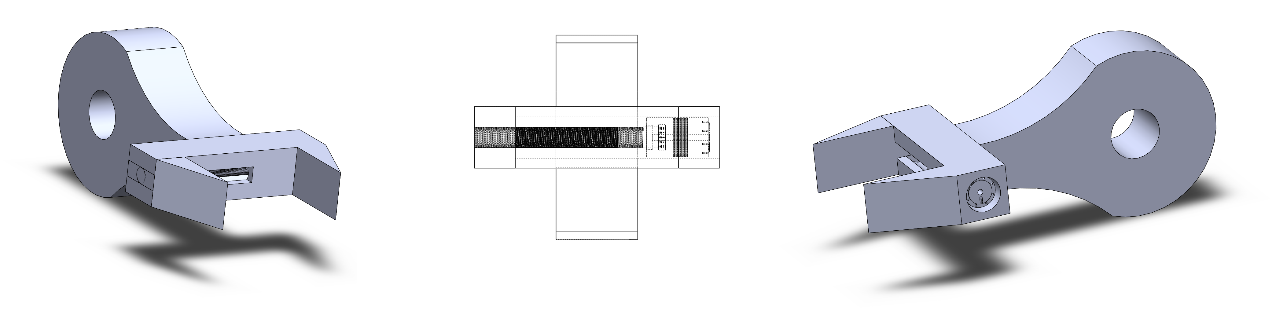
Robot Gripper

A gripper capable to hold a 80 mm square object is connected to frame $\{W\}$. In one of the gripper's claws there is a micro-motor to enable the gripper to hold. One of the claws of the gripper is attached to a threaded cylinder and then attached to a micro-motor, which will rotate the threaded cylinder and make the claw move. The Figure below shows the details of the gripper.

Entire Model

Together with the Arms and the Gripper there is a fixed base and a rotational base. The Soliworks model shown on Figure \ref{Model} the electronics are discussed on the next topic.

Other Components

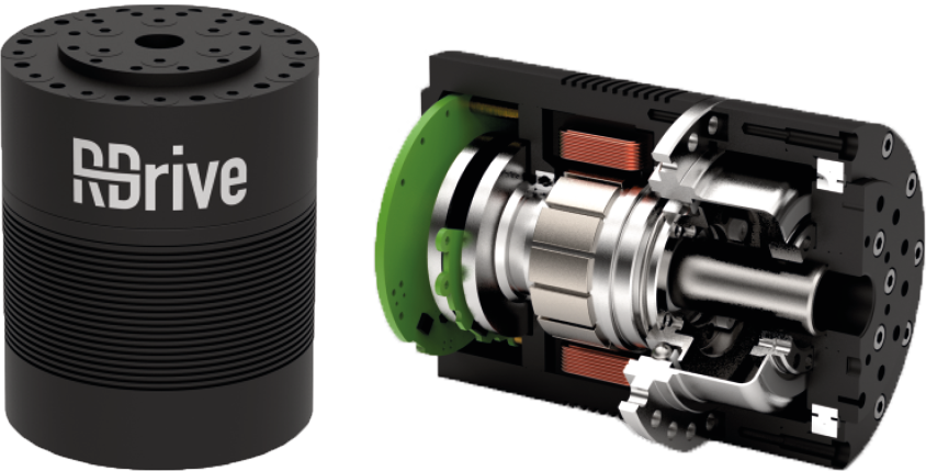
The actuator chosen for the project is a complete system with sensors, controller and a motor. It can be used on several applications such as robots and drones, model aircrafts, conveyor belts, sorting and assembly lines, and packing equipment to name some.

Motors

There are various types of motors and key factors need to be taken into account when selecting one for a particular application [3], in this case to control the joints of a robotic manipulator. The main factors are:

Inertia matching

The robotic system have to be capable to achieve a required torque to give a load a moment of particular inertia and to achieve a desired angular acceleration. The moment of inertia was calculated using the Iterative Newton-Euler Dynamics Algorithm [7], and this is solved in two parts, first the links velocities and accelerations are iteratively computed across the links applying the Newton-Euler equations to each link, then the forces and torques of interaction and joint actuator torques are computed recursively from the last link to the first.

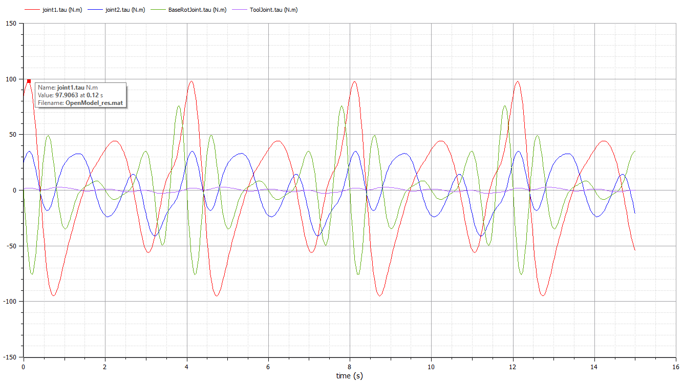
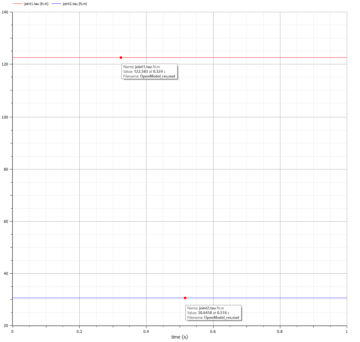
This calculation was made by simulating the system using a simulation software, OpenModelica. The values for $\tau$ of each joint during the time of the simulation, $15 s$, are shown on the Figure below, and, as can be noted, the maximum torque required was $97.9063 N.m$. The simulation was made with the load attached to the system.

Torque requirements

High torque means a mechanism is able to handle heavier loads. The motor used for the modelling is capable of $157 N.m$ and should be able to handle the $97.9063 N.m$ with a $59.0937 N.m$ margin.

Power requirements

As well as the torque requirements this project don't require that the motors run at maximum velocity, therefore overheating will not be a problem, and this is one of the main aspects of power requirements for a motor. The total power required is the sum of the power needed to overcome friction and that needed to accelerate the load [4].

After analysing and taking into consideration the aspects discussed above the RDrive 85 motor with rated torque of $108 N.m$ and peak torque of $157 N.m$ and $450W$ of Power was chosen to the task. [8] For the gripper a 20 mm diameter motor was used.

Sensors

To know the angular position of the joints absolute encoders shall be the choice because they give the actual angular position, a unique identification of an angle. The incremental encoders would detect the changes but in relation to some Datum. [3]

So with the absolute encoders we can track $\theta_1,\theta_2$, $\theta_3$ and $\theta_4$ and rearrange the links accordingly with the joints angles.

Also a loading cell can be used on the toll to sense the amount of pressure to set a trigger to avoid damage on the object.

Controllers

The final printed size of an author photograph is exactly 1 inch wide by 1 1/4 inches long (6 picas~$\times$~7 1/2 picas). Please ensure that the author photographs you submit are proportioned similarly. If the author's photograph does not appear at the end of the paper, then please size it so that it is proportional to the standard size of 1 9/16 inches wide by 2 inches long (9 1/2 picas~$\times$~12 picas). JPEG files are only accepted for author photos.

Control Methodology

IEEE accepts color graphics in the following formats: EPS, PS, TIFF, Word, PowerPoint, Excel, and PDF. The resolution of a RGB color TIFF file should be 400 dpi.

When sending color graphics, please supply a high quality hard copy or PDF proof of each image. If we cannot achieve a satisfactory color match using the electronic version of your files, we will have your hard copy scanned. Any of the files types you provide will be converted to RGB color EPS files.

Forward Kinematic

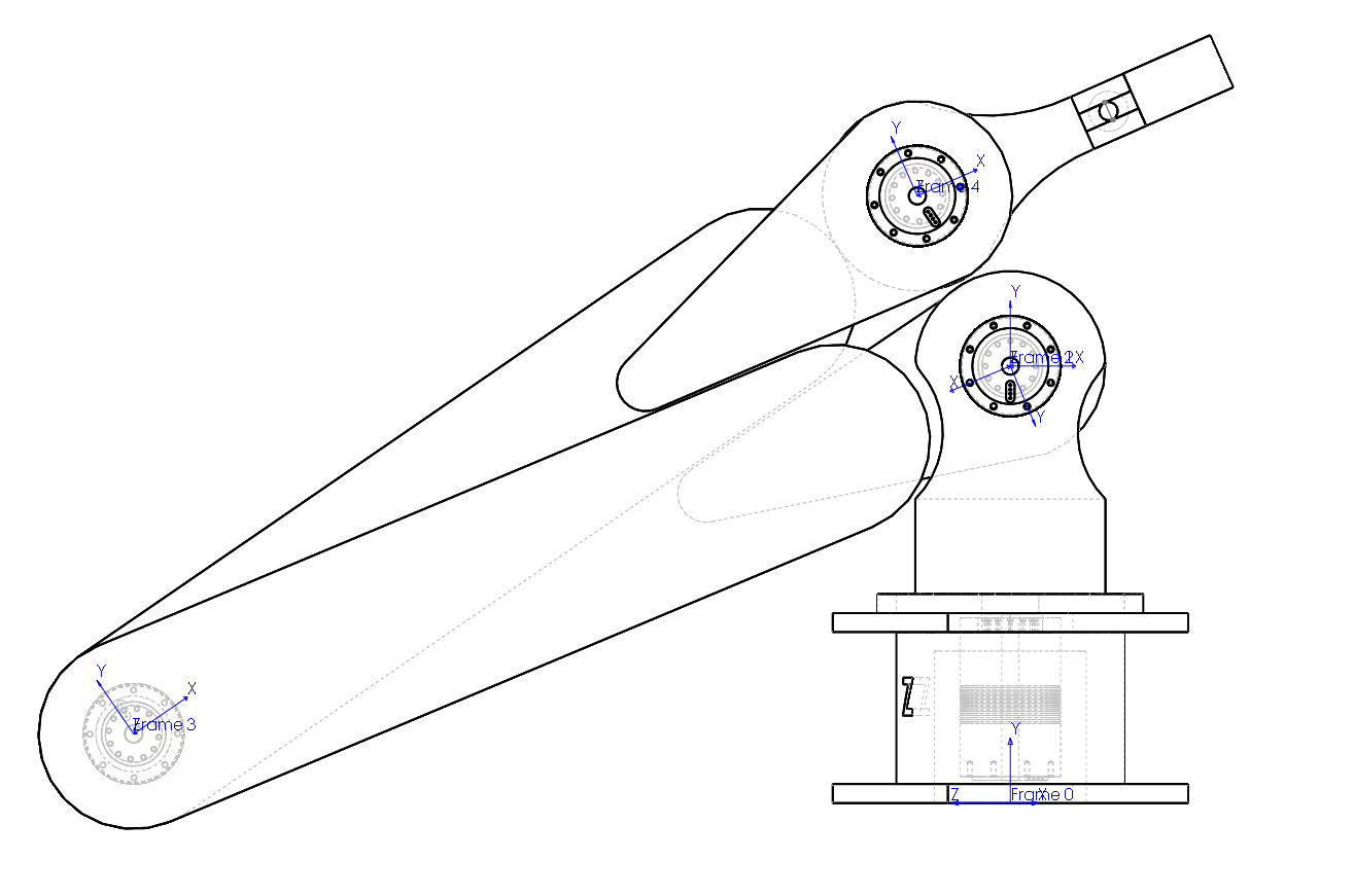
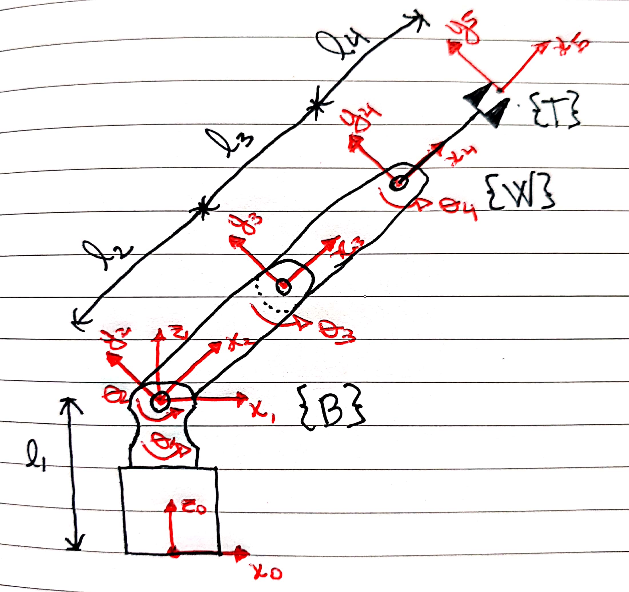
To calculate the forward kinematics equation, a Python Class called "FowardKinematics" was created, this Class has two main methods involved on the calculations, the rotation and the translation for the $\hat Z$ and $\hat X$ axis. The parameters for these methods are extracted from the Denavit–Hartenberg parameters at $(1)$, the coordinate systems and also the basic frames $\{B\}$, $\{W\}$ and $\{T\}$, Base, Wrist and Tools respectively are identified on the Figure below. The size of the links are $l_1 = 230$, $l_2 = 500$, $l_3 = 500$, $l_4 = 180$.

The forward kinematics calculations were confirmed by a python programming code that can be found in the Appendix A.

The rotation method receives an argument $self$ and $\theta_i$ for the rotation on the $\hat Z$ axis and $\alpha_{i-1}$ for $\hat X$. The $self$ argument is what makes this a method and not just a plain function, this is filled in automatically, when we call this method on the object. So we'll just provide one argument, and the fact that it's being called on the method will provide the first argument, self. It will then build a $sympy$ symbolic matrix and passes the $self$ argument to the method to be put in place, if no arguments are passed default values will be put in place as specified in the key word arguments (\** $kwargs$) on the $\_\_init\_\_$ function. A Matrix is then returned after calling the $.evalf()$ function to evaluate.

Like in the rotation method the translation method receives a argument $d_i$ and $a_{i-1}$ to return a matrix that translates in $\hat Z$ and $\hat X$ axis respectively. This class is also detailed in the Appendix A.

The objective of the forward kinematics is to provide a kinematics equation relating the end-effector orientation and position. This is done by finding the Denavit–Hartenberg parameters and the homogeneous transforms for each step from 0 to 5. These matrix are shown from (2) to (09). Finally, the forward kinematics equation is presented on Equation 9.

Finally, the forward kinematics equation is presented on Equation 8.

i	$\alpha_{i-1}$	$a_{i-1}$	$d_i$	$\theta_i$
1	0	0	$l_1$	$\theta_1$
2	$90^{\circ}$	0	0	$\theta_2$
3	0	$l_2$	0	$\theta_3$
4	0	$l_3$	0	$\theta_4$
5	0	$l_4$	0	0

Denavit–Hartenberg parameters (2)

$^0_1T = \begin{bmatrix} cos\theta_1 & -sin\theta_1 & 0 & 0 \\ sin\theta_1 & cos\theta_1 & 0 & 0 \\ 0 & 0 & 1 & l_1 \\ 0 & 0 & 0 & 1 \\ \end{bmatrix} \qquad(3)$

$^1_2T = \begin{bmatrix} cos\theta_2 & -sin\theta_2 & 0 & 0 \\ 0 & 0 & -1 & 0 \\ sin\theta_2 & cos\theta_2 & 0 & 0 \\ 0 & 0 & 0 & 1 \\ \end{bmatrix} \qquad(4)$

$^2_3T = \begin{bmatrix} cos\theta_3 & -sin\theta_3 & 0 & l_2 \\ sin\theta_3 & cos\theta_3 & 0 & 0 \\ 0 & 0 & 1 & 0 \\ 0 & 0 & 0 & 1 \\ \end{bmatrix} \qquad(5)$

$^3_4T = \begin{bmatrix} cos\theta_4 & -sin\theta_4 & 0 & l_3 \\ sin\theta_4 & cos\theta_4 & 0 & 0 \\ 0 & 0 & 1 & 0 \\ 0 & 0 & 0 & 1 \\ \end{bmatrix} \qquad(6)$

$^4_5T = \begin{bmatrix} 1 & 0 & 0 & l_4 \\ 0 & 1 & 0 & 0 \\ 0 & 0 & 1 & 0 \\ 0 & 0 & 0 & 1 \\ \end{bmatrix} \qquad(7)$

$^0_5T = ^0_1T ^1_2T ^2_3T ^3_4T ^4_5T => ^0 \cancel{_1T ^1_2T ^2_3T ^3_4T ^4} _5T = ^0_5T \qquad(8)$

$^0_5T = \begin{bmatrix} C_1C_{234} & -S_{234}C_1 & S_1 & C_1(l_2 C_2 + l_3 C_{23} + l_4 C_{234}) \\ &&&& \\ S_1 C_{234} & -S_1 S_{234} & -C_1 & S_1 (l_2 C_2 + l_3 C_{23} + l_4 C_{234}) \\ &&&& \\ S_{234} & C_{234} & 0 & l_1 + l_2 S_2 + l_3 S_{23} + l_4 S_{234} \\ &&&& \\ 0 & 0 & 0 & 1 \\ \end{bmatrix} \qquad(9)$

Inverse Kinematics

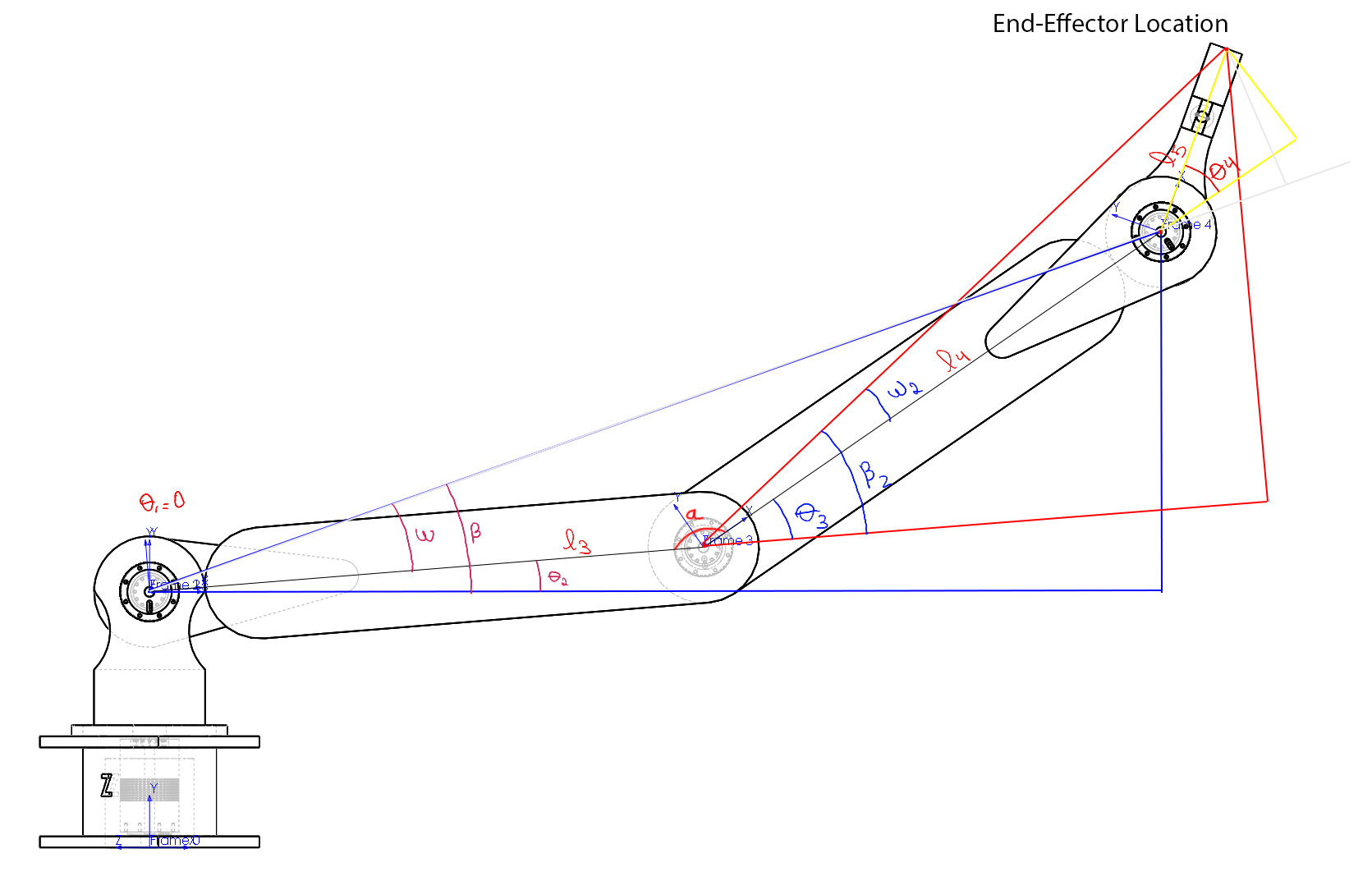
There are many methods to find the equations for the inverse kinematic here two methodologies are presented. First let's look at the trigonometric solution. For the trigonometric solution we can draw 2 triangles, on from frame $\{1\}$ to $\{4\}$ and the second one from frame $\{3\}$ to frame $\{5\}$. This way we can study the relation between the angles.

If we assume $theta_1 = 0$ we can calculate the angle relation between the triangles on Figure below as if they were on the same plane.

To find the hypotenuses of the triangles we have to find $^1_4T$, $^3_5T$ and $^1_5T$. This can be achieved by multiplying both sides of Equation 10 by the dependent transpose inverse $T^{-1}$, as shown below.

If we consider Equation 8:

$^0_5T = ^0_1T ^1_2T ^2_3T ^3_4T ^4_5T \qquad(10)$

and we multiply both sides by $^0_1T^{-1}$ we have,

$^0_5T {^0_1T}^{-1} = {^0_1T}^{-1} {^0_1T} ^1_2T ^2_3T ^3_4T ^4_5T \qquad(11)$

Which is the same as,

$^1_5T = ^1_2T ^2_3T ^3_4T ^4_5T \qquad(12)$

To find $^1_4T$ we can "go" to $^1_5T$ and "coming back" one step by computing the inverse $^4_5T^{-1}$. Then we have,

$^1_4T = ^1_5T ^4_5T^{-1} \qquad(13)$

And for $^3_5T$ from the red triangle we can multiply $^1_2T^{-1}$ and $^2_3T^{-1}$ by $^1_5T$. Then we have,

$^3_5T = ^1_5T {^1_2T}^{-1} {^2_3T}^{-1} \qquad(14)$

Computing $^1_4T$, calculation made on Appendix A,

$^1_4T = \begin{bmatrix} C_{234} & -S_{234} & 0 & l_2 C_2 + l_3 C_{23} \\ 0 & 0 & -1 & 0 \\ S_{234} & C_{234} & 0 & l_2 S_2 + l_3 S_{23} \\ 0 & 0 & -1 & 1 \\ \end{bmatrix} \qquad(15)$

And $^3_5T$,

$\begin{matrix} ^3_5T = \begin{bmatrix} C_{3}C_{34} & S_{3}C_{34} & -S_{34} & l_2 C_2 - l_2 C_3 C_{34} + L_3 C_{23} + L_4 C_{234} \\ -S_3 & C_3 & 0 & l_2 S_3 \\ S_{34} C_3 & S_3 S_{34} & cos_{34} & l_2 S_2 - l_2 C_3 S_{34} + L_3 S_{23} + L_4 S_{234}\\ 0 & 0 & -1 & 1 \\ \end{bmatrix} \end{matrix} \qquad(16)$

By using the law of cosines which states that, on a triangle $A, B, C$, we have,

$\begin{matrix} c^2 = \vec{c} . \vec{c} = \\ (\vec{b} - \vec{a}).(\vec{b} - \vec{a}) = \\ b^2 + a^2 - 2\vec{a} . \vec{b} = \\ b^2 + a^2 - 2 ab cosC. \end{matrix} \qquad(17)$

Applying to the blue triangle on the Figure below,

$\begin{matrix} cos\omega = \frac{l_4^2 - l_3^2 - x^2 - y^2}{-2l_3 \sqrt{x^2 + y^2}} \\ \\ sin \omega = \sqrt{1 - {cos \omega}^2} \end{matrix} \qquad(18)$

Therefore,

$\begin{matrix} \beta = Atan2(x_{15}, y_{15}) \\ \theta_2 = \beta - \omega \end{matrix} \qquad(19)$

Applying the same to the red triangle and considering $(x, y)$ as from $^3_5T$, we have,

$\begin{matrix} l_5^2 = l_4^2 + {\sqrt{x^2 + y^2}}^2 - 2 l_4 \sqrt{x^2 + y^2} cos \omega_2 =\\ \\ cos \omega_2 = \frac{l_5^2 - l_4^2 - x^2 - y^2}{-2l_4 \sqrt{x^2 + y^2}} \\ \\ sin \omega_2 = \sqrt{1 - {cos \omega_2}^2} \end{matrix} \qquad(20)$

Therefore,

$\begin{matrix} \beta_2 = Atan2(x_{35}, y_{35}) \\ \theta_3 = \beta_2 - \omega_2 \end{matrix} \qquad(21)$

For $\theta_4$ we have,

$\theta_4$ = $Atang(x_{14}, y_{14}) +$ $\frac{l_3^2 - l_2^2 - x_{14}^2 - y_{14}^2} {-2l_2 \sqrt{x_{14}^2 + y_{14}^2}} \qquad(22)$

As a proof of the equations for the inverse kinematics a program in python was written using the a simple case where $\theta_2 = 0$, $\theta_2 = 45$ and $\theta_4 = 45$. The results were consistent and the program is exposed on Appendix A.

System Simulation

OpenModelica is currently the most complete open-source Modelica and FMI based modelling, simulation, optimization, and model-based development environment. Its long-term development is supported by a non-profit organization – the Open Source Modelica Consortium (OSMC). [2]

This system was chosen, mainly, because of the open-source aspect, since Mathworks Simulink requires a paid plugin to connect the Solidworks model. Also due to the fact that Its a complete system for simulation modelling, versatile and capable of very complex tasks, much more complex than the current project.

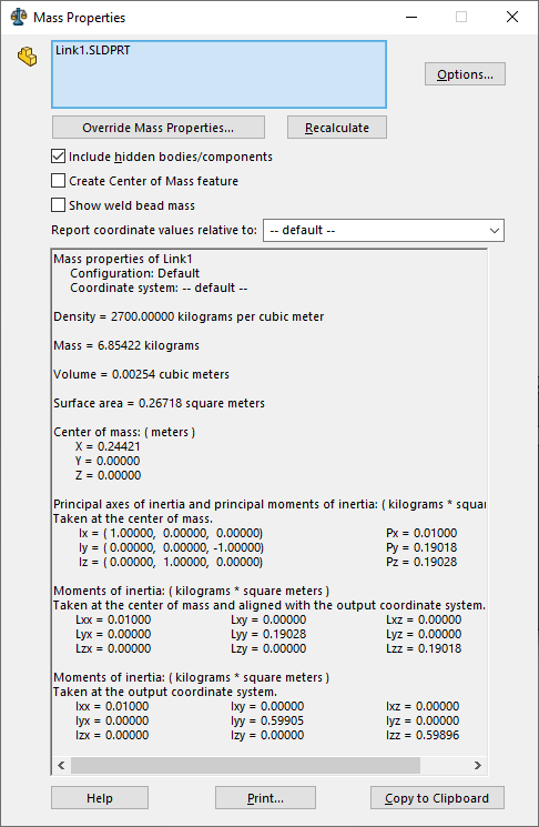
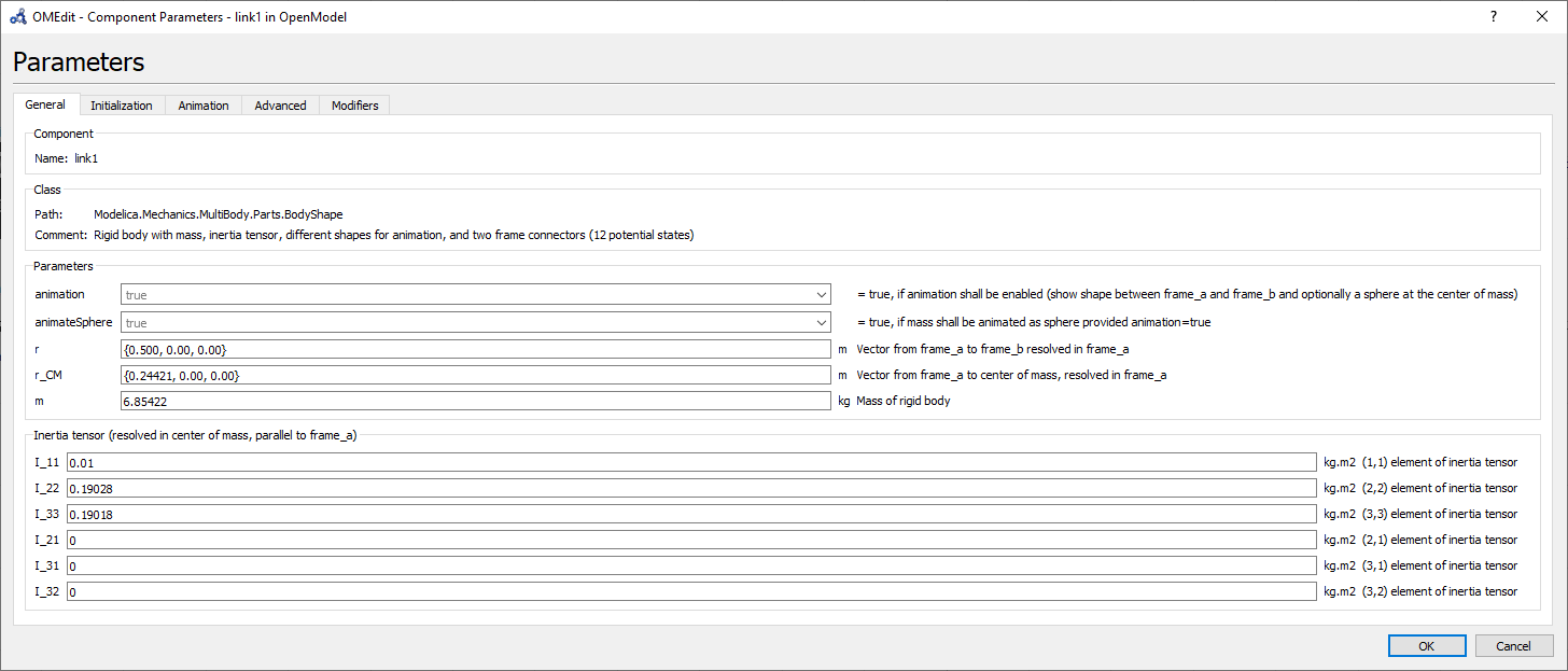
For the modelling simulation parameters, information from the CAD simulator (SolidWorks) regarding to mass, center of mass and moments of inertia, were confronted with the Python simulation and was consistent as shown on the Figure below and at the Python programming documentation that can be found on Appendix A. More information about the model is also provided but not included necessary to the link properties at OpenModelica, like density, volume, surface area, among others. The parameters necessary for the model were the length, mass and center of mass, as well as the inertia tensors, as shown on the Figure below.

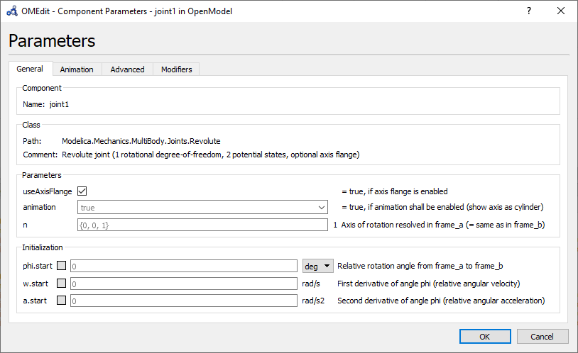
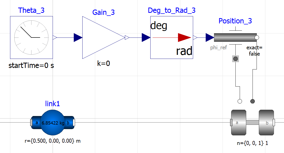
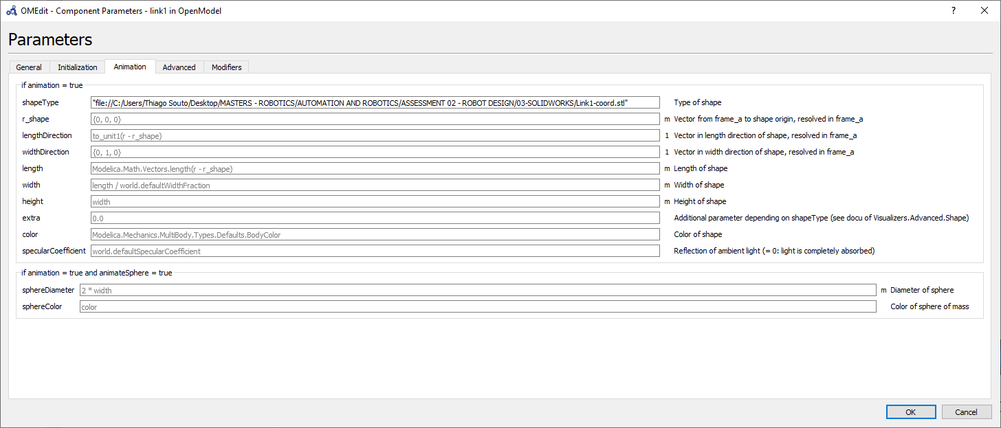
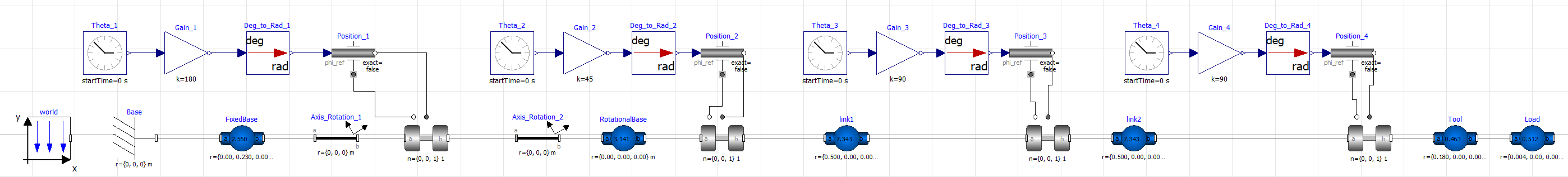
To simulate the manipulator the component $Joints.Revolute$ was used for the joints, and $Parts.BodyShapes$ was used for the links, base and tool, and also some auxiliary component blocks to simulate controllers, world conditions and a fixed base (ground). On the $Joints.Revolute$ component for the joints the option $useAxisFlange$, allow the control of the rotation and this option was used as shown on the $joint1$ parameters on the Figure below. A unit conversion block has to be used to convert from degrees to radians, there is a math block for that. With this control system the position can provide for $joint1$ by setting a value to the $Gain$ block. This will take the gain input and will provide it as a signal that the joint can use. This 6 blocks represent the first joint link of the system as represented on the Figure below.

The CAD modeling software chosen was SolidWorks from Dassault Systems, It is a solid modeling computer-aided design software with 2.3 million active users at over 234,800 companies in 80 countries. [5] SolidWorks goal is building 3D CAD software that was easy-to-use, affordable, and available on Windows. [6] The main reasons to use SolidWorks in this project were the easy of use, the calculations that can be used as OpenModelica parameters and the exporting features that allows easy integration between the two software.

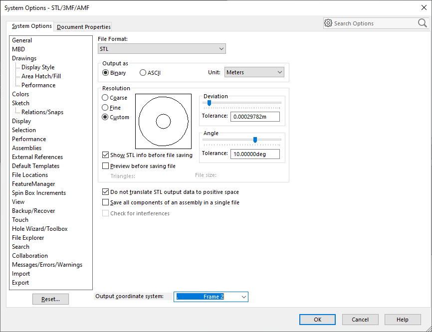
An import aspect of exporting from Solidworks to OpenModelica is the compatibility, the exported file can be a $.STL$ file. Although the measurements have to be in meters. In the $STL$ exporting window there is the option "Do not translate $STL$ output data to positive space", this option makes exported parts maintain their original position in global space, relative to the origin [4].

There are many ways to export from one software to the other, on this project approach, at the export STL window, the coordinate system is been output, as can be seen in the import parameters for link 1 on the Figure below, by exporting the coordinate system placed on the frame position, also on the following Figure below, the vector from frame $\{A\}$ to the shape origin, resolved in $\{A\}$ is equal to 0, because the frame coordinate system exported is located at the origin.

We can use the center of mass directly from SoildWorks as well as use the exact distance between the frames at the $r$ parameter as shown on the next Figures.

The calculations for the moments of inertia were made in Python, refer to Appendix A, and confirmed in the mass evaluation at SolidWorks, also, in OpenModelica, as can be seen see on the Figure below the values for the torque for joint 1 and 2 using $\theta_{1-4}$ = $0^{\circ}$.

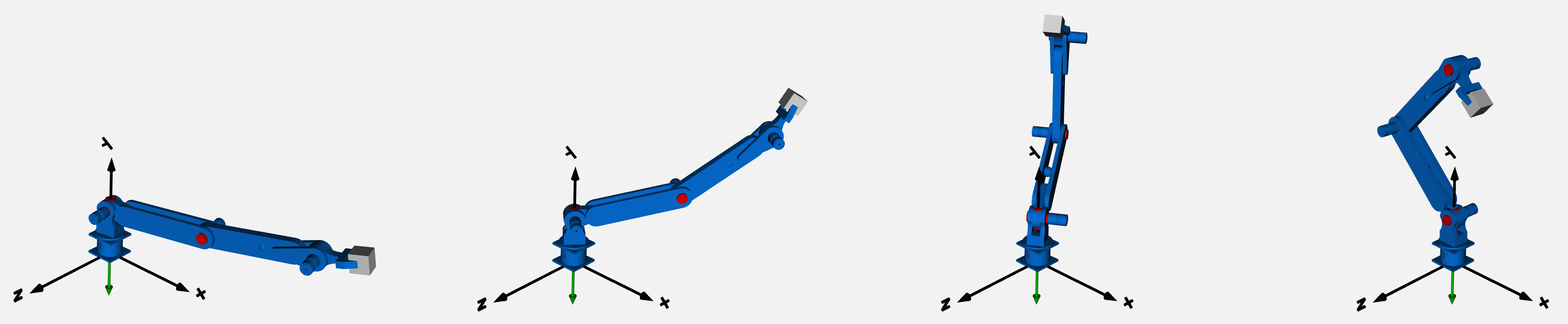
Here the simulation modelling at OpenModelica is shown, the parameters used at the $Gain$ block results in an animation, that goes from all the angles been 0 to the values set.

Solidworks simulation

A Solidworks simulation of the manipulator picking a box on a conveyor and placing it in another conveyor is shown below.

Discussion and Conclusions

Robot manipulators are huge contributor for the robot revolution and will continue to push the industry ahead. The study of it's components and the interactions between them are very important to predict if the designed manipulator will be able to accomplish the task for what it is purposed. New tools for simulation of these robots are improving every day and with such tools, in this project, we were able to demonstrate the design of a robotic manipulator capable of picking objects as well as its forward and inverse kinematics equations. Further developments will include an interface to control the manipulator with real time calculations displayed with the aim of better understand the variables of such an interesting and important tool.

Bibliography

1. J. J. Craig, \emph{Introduction To Robotics: Mechanics And Control}, 3rd ed., Ed. New York: Pearson Education, 2009.
2. P. Fritzson, et al. \emph{The OpenModelica Integrated Modeling, Simulation and Optimization Environment} (Conference paper), PROCEEDINGS OF THE 1ST AMERICAN MODELICA CONFERENCE$. $Cambridge, USA: Massechusetts, 2018.
3. W. Bolton, \emph{Mechatronics - Electronic control systems in mechanical and electrical engineering}. United Kingdom: Pearson Education Limited, 2019.
4. (SOLIDWORKS Online Help) Dassault Systems. (2020, May). Available: https://help.solidworks.com/.
5. (The SOLIDWORKS blog) Dassault Systems. (2020, May). Available: https://blogs.solidworks.com/solidworksblog/2016/10/growing-solidworks-nation.html.
6. (SolidWoks - Wikipedia)(2020, May). Available: https://en.wikipedia.org/wiki/SolidWorks.
7. K.N. Frazer, School of Food and Advanced Technology, Massey University, Slides from Lecture 12, March 2019.
8. \emph{RDrive Datasheet} ROZUM Robotics LLC., Mountain House, CA - USA, 2020.
9. (Atan2 - Wikipedia)(2020, May). Available: https://en.wikipedia.org/wiki/Atan2

Appendix A

To Appendix A please follow the link.